Play with MNIST and tensorflow 2.1
In this post we use tensorflow 2.1 custom model and custom loop on the famous MNIST dataset. We perform a multiclass classification with a basic convolutional neural network.
According to offical website, MNIST dataset is a database of handwritten digits. It contains a training and a test set. The digits have been size-normalized and centered in a fixed-size image.
It is a good database for people who want to try learning techniques and pattern recognition methods on real-world data while spending minimal efforts on preprocessing and formatting.
This dataset contains 10 classes (digits from 0 to 9) and images are in the grayscale (1-channel). As a reminder color images have three 3 channels: red, green and blue.
Here is a link to the notebook.
Let’s get started !
Load useful packages
import tensorflow as tf
from tensorflow.keras.layers import Dense, Flatten, Conv2D, Reshape, MaxPooling2D
from tensorflow.keras import Model

import numpy as np
import matplotlib.pyplot as plt
import pandas as pd
from sklearn.metrics import confusion_matrix
import seaborn as sns
Data preparation and exploration
Load the dataset
# Load
mnist_dataset = tf.keras.datasets.mnist.load_data()
# Unpack
(x_train, y_train), (x_test, y_test) = mnist_dataset

# Train dataset shapes
print('Train X shape ', x_train.shape)
print('Train Y shape ', y_train.shape)
#=> Train X shape  (60000, 28, 28)
#=> Train Y shape  (60000,)
# Test dataset shapes
print('Test X shape ', x_test.shape)
print('Test Y shape ', y_test.shape)
#=> Test X shape  (10000, 28, 28)
#=> Test Y shape  (10000,)
Explore images
print("pixel unique values:", len(np.unique(x_train)),
      "\nmin value:", np.min(x_train),
      "\nmax value:", np.max(x_train))
#=> pixel unique values: 256
#=> min value: 0
#=> max value: 255
Explore labels
print("unique labels:", len(np.unique(y_train)),
      "\nmin value:", np.min(y_train),
      "\nmax value:", np.max(y_train))
#=> unique labels: 10
#=> min value: 0
#=> max value: 9
Inspect density probability distribution over the training/test sets
see code ref: datasets_distribution, print_dataset_distributions
We plot an histogram of the label distributions to see how balanced are the labels among samples, and among the training and test set.
traintest = datasets_distribution(y_train, y_test)
print(traintest)
print_dataset_distributions(traintest)
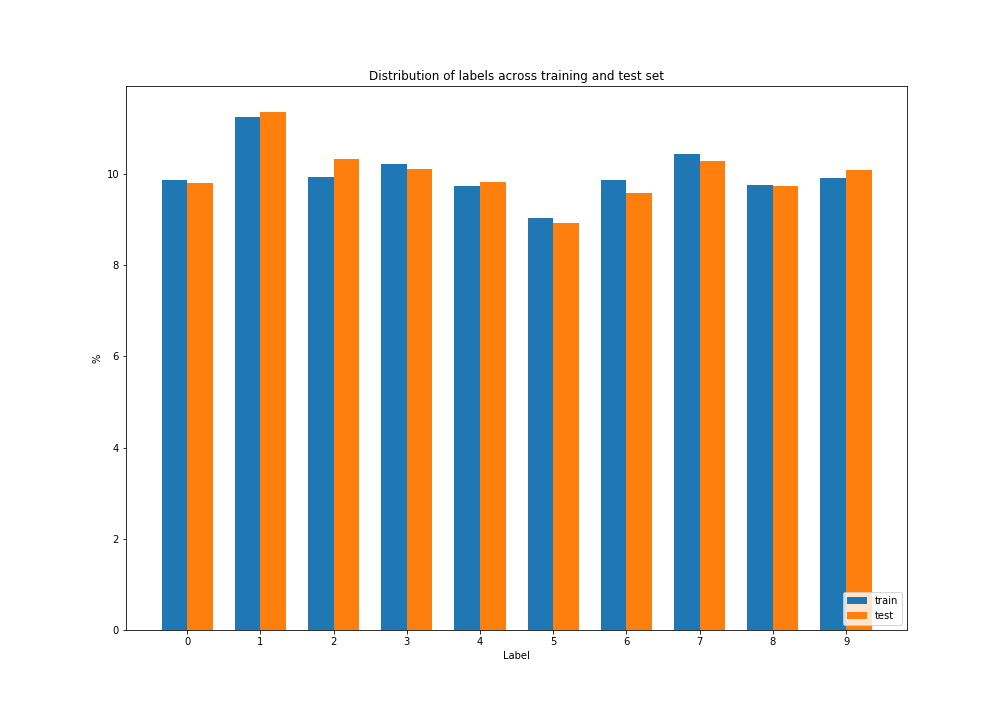
| label | train (%) | test (%) |
|---|---|---|
| 0 | 9.871667 | 9.80 |
| 1 | 11.236667 | 11.35 |
| 2 | 9.930000 | 10.32 |
| 3 | 10.218333 | 10.10 |
| 4 | 9.736667 | 9.82 |
| 5 | 9.035000 | 8.92 |
| 6 | 9.863333 | 9.58 |
| 7 | 10.441667 | 10.28 |
| 8 | 9.751667 | 9.74 |
| 9 | 9.915000 | 10.09 |
We can see that:
- distribution among labels are pretty close
- distribution for the training set and the test set are also very close.
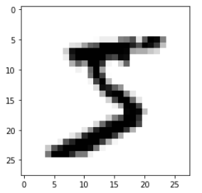
Show me an image
see code ref: show_image
show_image(x_train, 0)
Gather and prepare
see code ref: prepare_mnist_dataset
Here, we prepare the samples by converting them from integers (0-255) to floating-point numbers (0.0-1.0). Then we have to reshape the samples to fit in the convolutional layer. Thus, we add one dimension, because the first convolutional layer expect a 4D tensor ([batch, in_height, in_width, in_channels]).
def prepare_mnist_dataset(mnist_dataset):
  """
  Get the data form MNIST dataset
  http://yann.lecun.com/exdb/mnist/
  :param mnist_dataset: MNIST dataset
  :return: tuple containing (x_train, y_train), (x_test, y_test)
  """
  (x_train, y_train), (x_test, y_test) = mnist_dataset
  # Reduce the samples from integers
  x_train, x_test = x_train / np.float32(255), x_test / np.float32(255)
  y_train, y_test = y_train.astype(np.int64), y_test.astype(np.int64)
  # Get the number of training and test samples
  m_train = x_train.shape[0]
  m_test = x_test.shape[0]
  # Get image dimensions
  height = x_test.shape[1]
  width = x_test.shape[2]
  # Reshape adding one dimension for the channel
  x_train = x_train.reshape(m_train, height, width, 1)
  x_test = x_test.reshape(m_test, height, width, 1)
  return (x_train, y_train), (x_test, y_test)
Define the model
see code ref: SimpleConvModel, tf.keras.layers.Conv2D, tf.keras.layers.MaxPool2D, tf.keras.layers.Flatten, tf.keras.Model
We define a custom tensorflow model by creating a class that inherits from tf.keras.Model.
In this class, we build a sequencial neural network with the help of some predefined keras layers:
-
Conv2D(32, (3,3), input_shape=(28, 28, 1), activation="relu")- a 2D convolutional layer for spatial convolution over an image
- channel: only one has the input is grey colour
- convolutions: 32, size of the convolution 3x3 grid
- activation function: ReLU
-
MaxPooling2D(2, 2)- a MaxPooling layer that compress the image while maintaining the content of the features that were highlighted by the convolution.
- size: (2,2) the effect is to quarter the size of the image.
class SimpleConvModel(Model):
  """
  Custom convolutional model
  """
  def __init__(self, image_height, image_width, channel_count):
    """
    Constructor
    :param self: self
    :param image_height: height of image in pixel
    :param image_width: width of image in pixel
    :channel_count: channel count, for example color image has 3 channels, grayscale image has only one channel
    :return: void
    """
    super(SimpleConvModel, self).__init__()

    # Define sequential layers
    self.convolution = Conv2D(32, (3,3), input_shape=(image_height, image_width, channel_count), activation="relu")
    self.max_pooling = MaxPooling2D(2, 2)
    self.flatten = Flatten()
    self.dense = Dense(128, activation="relu")
    self.softmax = Dense(10, activation="softmax")

    # Keep convolutional layer output
    self.convolutional_output = tf.constant(0)
    # Keep max pooling layer output
    self.max_pooling_output = tf.constant(0)
    # Input signature for tf.saved_model.save()
    self.input_signature = tf.TensorSpec(shape=[None, image_height, image_width, channel_count], dtype=tf.float32, name='prev_img')

  def call(self, inputs):
    """
    Forward propagation
    :param self: self
    :param inputs: tensor of dimension [batch_size, image_height, image_width, channel_count]
    :return: predictions
    """
    self.convolutional_output = self.convolution(inputs)
    self.max_pooling_output = self.max_pooling(self.convolutional_output)
    x = self.flatten(self.max_pooling_output)
    x = self.dense(x)
    return self.softmax(x)
Then we create a SimpleConvModel to see more details about the neural network we’ve just built.
# Create a model instance
IMAGE_HEIGHT = 28
IMAGE_WIDTH = 28

model = SimpleConvModel(IMAGE_HEIGHT, IMAGE_WIDTH, 1)
model.build(input_shape=(None, IMAGE_HEIGHT, IMAGE_WIDTH, 1))
model.summary()
#=> Model: "simple_conv_model"
#=> _________________________________________________________________
#=> Layer (type)                 Output Shape              Param #
#=> =================================================================
#=> conv2d (Conv2D)              multiple                  320
#=> _________________________________________________________________
#=> max_pooling2d (MaxPooling2D) multiple                  0
#=> _________________________________________________________________
#=> flatten (Flatten)            multiple                  0
#=> _________________________________________________________________
#=> dense (Dense)                multiple                  692352
#=> _________________________________________________________________
#=> dense_1 (Dense)              multiple                  1290
#=> =================================================================
#=> Total params: 693,962
#=> Trainable params: 693,962
#=> Non-trainable params: 0
#=> _________________________________________________________________
For better understanding of the tensorflow output, here is a table where we added the input and output dimensions. To simplifiy, we omit the batch/sample size.
| Layer | Input Dimension | Output Dimension | Parameter Count |
|---|---|---|---|
| Conv2D | 28x28 | 32x26x26 | (3x3 + 1) x 32 |
| MaxPooling2D | 32x26x26 | 32x13x13 | 0 |
| Flatten | 32x13x13 | 5408 | 0 |
| Dense (128) | 5408 | 128 | (5408 + 1) x 128 |
| Dense softmax (10) | 128 | 10 | (128 + 1) x 10 |
For the first layer, we have 32 filters of square size 3x3. Each filter has 9 parameters (3x3). So then the number of parameter is (9 + 1) by 32 because we add the bias unit for every filter.
Optimizer
see code ref: tf.keras.optimizers.Adam()
We choose ADAM optimizer for (Adaptive Moment Estimation). It is a combination of AdaGrad and RMSProp algorithm.
optimizer_function = tf.keras.optimizers.Adam()
Loss
see code ref: tf.keras.losses.SparseCategoricalCrossentropy
Computes the crossentropy loss between the labels and predictions. For more information go to section “\(\mathcal{L}\) as Loss function and \(E\) as Error” in my previous post
loss_function = tf.keras.losses.SparseCategoricalCrossentropy()

def compute_loss(labels, logits):
  """
  Compute loss
  :param labels: true label
  :param logits: predicted label
  :return: loss
  """
  return loss_function(labels, logits)
Accuracy
see code ref: tf.math.argmax, tf.math.reduce_mean, tf.cast, tf.math.equal
Accuracy is the first metric we usually computes. It represents the part of correct predictions.
def compute_accuracy(labels, logits):
  """
  Compute accuracy
  :param labels: true label
  :param logits: predicted label
  :return: accuracy of type float
  """
  predictions = tf.math.argmax(logits, axis=1)
  return tf.math.reduce_mean(tf.cast(tf.math.equal(predictions, labels), tf.float32))
Now, action ! 
Get the data prepared
see code ref: prepare_mnist_dataset, batch_dataset
# Prepare data
(x_train, y_train), (x_test, y_test) = prepare_mnist_dataset(mnist_dataset)

# Train
# Get a `TensorSliceDataset` object from `ndarray`s
train_dataset = tf.data.Dataset.from_tensor_slices((x_train, y_train))
train_dataset_batch = batch_dataset(train_dataset,
                        take_count = 60000,
                        batch_count = 100)

# Test
test_dataset = tf.data.Dataset.from_tensor_slices((x_test, y_test))
test_dataset_batch = test_dataset.batch(100)
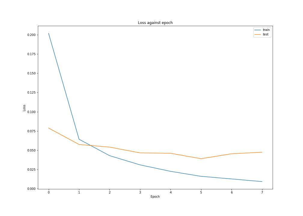
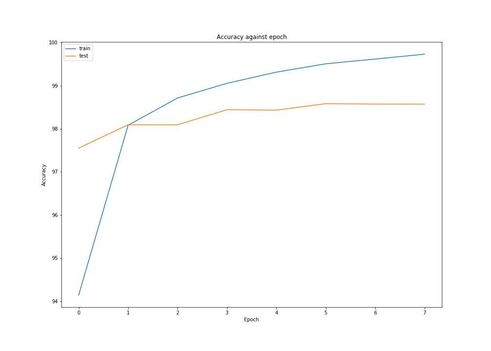
Optimization loop
see code ref: save, tf.keras.metrics.Mean, tf.keras.metrics.SparseCategoricalAccuracy, tf.GradientTape
We write an optimization loop helped by tf.GradientTape() which enables us to automatically computes the gradient. We stop the optimization loop when the test accuracy doesn’t improve for 2 epochs.
EPOCHS = 10

train_losses = []
train_accurarcies = []

test_losses = []
test_accurarcies = []

for epoch in range(EPOCHS):
  train_loss_aggregate = tf.keras.metrics.Mean(name="train_loss")
  test_loss_aggregate = tf.keras.metrics.Mean(name="test_loss")
  train_accuracy_aggregate = tf.keras.metrics.SparseCategoricalAccuracy(name="train_accuracy")
  test_accuracy_aggregate = tf.keras.metrics.SparseCategoricalAccuracy(name="test_accuracy")

  for train_images, train_labels in train_dataset_batch:
    with tf.GradientTape() as tape:
      # forward propagation
      predictions = model(train_images)
      # calculate loss
      loss = compute_loss(train_labels, predictions)

    # calculate gradients from model definition and loss
    gradients = tape.gradient(loss, model.trainable_variables)
    # update model from gradients
    optimizer_function.apply_gradients(zip(gradients, model.trainable_variables))

    train_loss_aggregate(loss)
    train_accuracy_aggregate(train_labels, predictions)

  for test_images, test_labels in test_dataset_batch:
    predictions = model(test_images)

    loss = compute_loss(test_labels, predictions)

    test_loss_aggregate(loss)
    test_accuracy_aggregate(test_labels, predictions)

  train_losses.append(train_loss_aggregate.result().numpy())
  train_accurarcies.append(train_accuracy_aggregate.result().numpy()*100)

  test_losses.append(test_loss_aggregate.result().numpy())
  test_accurarcies.append(test_accuracy_aggregate.result().numpy()*100)

  print('epoch', epoch,
        'train loss', train_losses[-1],
        'train accuracy', train_accurarcies[-1],
        'test loss', test_losses[-1],
        'test accuracy', test_accurarcies[-1])

  save(model, 'mnist/epoch/{0}'.format(epoch))

  if epoch > 1:
    if test_accurarcies[-2] >= test_accurarcies[-1] and test_accurarcies[-3] >= test_accurarcies[-2]:
      break
#=> epoch 0 train loss 0.2019603 train accuracy 94.14166808128357 test loss 0.07888014 test accuracy 97.54999876022339
#=> epoch 1 train loss 0.064292975 train accuracy 98.07999730110168 test loss 0.057503365 test accuracy 98.089998960495
#=> epoch 2 train loss 0.043002833 train accuracy 98.71166944503784 test loss 0.05409672 test accuracy 98.089998960495
#=> epoch 3 train loss 0.031002931 train accuracy 99.05166625976562 test loss 0.046595603 test accuracy 98.43999743461609
#=> epoch 4 train loss 0.022615613 train accuracy 99.31166768074036 test loss 0.04606781 test accuracy 98.43000173568726
#=> epoch 5 train loss 0.016122704 train accuracy 99.50500130653381 test loss 0.03901471 test accuracy 98.580002784729
#=> epoch 6 train loss 0.012739406 train accuracy 99.6150016784668 test loss 0.045439206 test accuracy 98.5700011253357
#=> epoch 7 train loss 0.009279974 train accuracy 99.72833395004272 test loss 0.047415126 test accuracy 98.5700011253357
It seems that the model begin to overfit after epoch 5 as the train accuracy still grow but the test accuracy begin to decrease.
For visualization, we plot the losses and accuracies over epochs.
see doc ref: losses, accuracies
Model evaluation
Confusion matrix, accuracy, precisions and recalls
see doc ref: custom_confusion_matrix, print_confusion, confusion_matrix
In real world problems, accuracy is not often a reliable metric for the performance of a classifier. Indeed, unbalanced data set will cause skewed accuracy results.
To overcome this, we often use confusion matrices, also called error matrices. In a confusion matrix the number of true/actual labels (by rows) are displayed against predicted labels (by columns). In this configuration, true positives (\(tp\)) are on the diagonal; false positive (\(fp\)) on columns; and false negative (\(fn\)) on rows.
| Pred. 0 | Pred. 1 | Pred. 2 | .. | Pred. 9 | Recall | |
|---|---|---|---|---|---|---|
| Act. 0 | Correct 0 | P=1 but A=0 | P=2 but A=0 | .. | P=9 but A=0 | Recall 0 |
| Act. 1 | P=0 but A=1 | Correct 1 | P=2 but A=1 | .. | P=9 but A=1 | Recall 1 |
| Act. 2 | P=0 but A=2 | P=1 but A=2 | Correct 2 | .. | P=9 but A=2 | Recall 2 |
| .. | .. | .. | .. | .. | .. | .. |
| Act. 9 | P=0 but A=9 | P=1 but A=9 | P=2 but A=9 | .. | Correct 9 | Recall 9 |
| Precision | Precision 0 | Precision 1 | Precision 2 | .. | Precision 9 | Accuracy |
We added three other metrics to the matrix: precision, accuracy and recall.
The accuracy is the percentage of predictions that are corrects, or the sum of all correct prediction over the total number of samples. Refering to the confusion matrix it’s the trace of the matrix over the total number of exemples.
\[accuracy = { Tr(confusion) \over m }\]Precision: when it predicts a k label, how often it is the true label.
\[precision(label = k) = { tp(label = k) \over tp(label = k) + fp(label = k) }\]Referring to the matrix, precisions can be calculated as follow
\[precisions = { diag(confusion) \over rowsum(confusion) }\]Recall or “true positive rate”, when it’s actually label k, how often does it predict label k
\[recall(label = k) = { tp(label = k) \over tp(label = k) + fn(label = k) }\]Referring to the matrix, recalls can be calculated as follow
\[recalls = { diag(confusion) \over colsum(confusion) }\]Remind the results of the optimization loop
| Epoch | train loss | train accuracy | test loss | test accuracy |
|---|---|---|---|---|
| 0 | 0.2019603 | 94.14166808128357 | 0.07888014 | 97.54999876022339 |
| 1 | 0.064292975 | 98.07999730110168 | 0.057503365 | 98.089998960495 |
| 2 | 0.043002833 | 98.71166944503784 | 0.05409672 | 98.089998960495 |
| 3 | 0.031002931 | 99.05166625976562 | 0.046595603 | 98.43999743461609 |
| 4 | 0.022615613 | 99.31166768074036 | 0.04606781 | 98.43000173568726 |
| 5 | 0.016122704 | 99.50500130653381 | 0.03901471 | 98.580002784729 |
| 6 | 0.012739406 | 99.6150016784668 | 0.045439206 | 98.5700011253357 |
| 7 | 0.009279974 | 99.72833395004272 | 0.047415126 | 98.5700011253357 |
We focus on epoch n°0 and n°5 which are the two most different epochs in terms of accuracies.
Here is the confusion matrix for epoch 0:
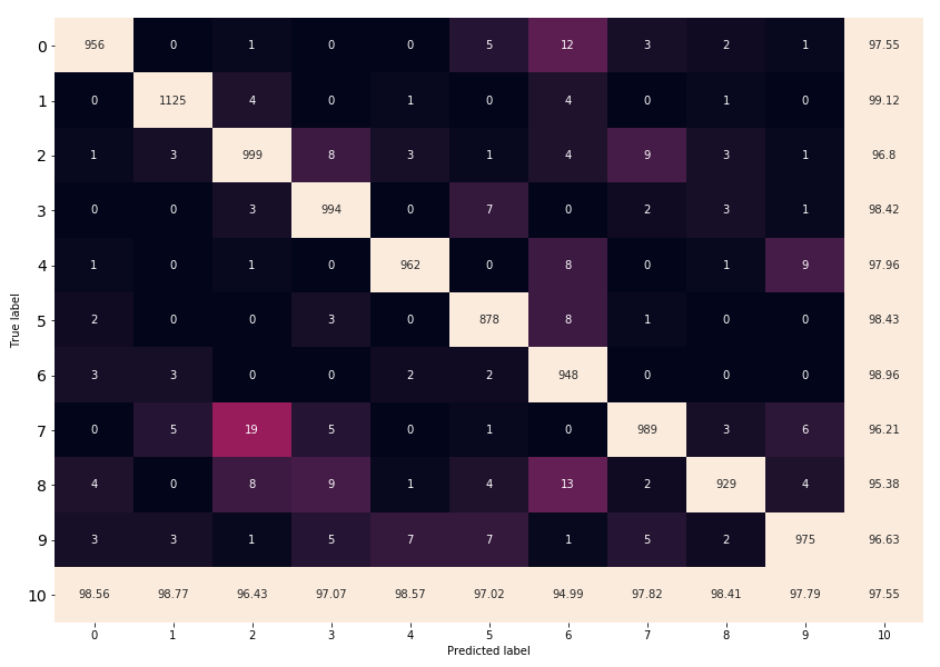
We can see that 19 images are misclassified 2 instead of 7.
For epoch 5
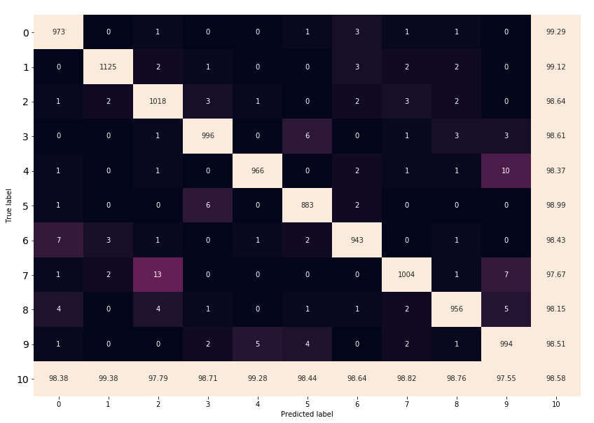
Here again a significant number of 7 are misclassified as 2. Indeed, the label 7 has the poorest recall rate.
We also notice that in general true labels 2 are correctly classified.
On the other side, label 9 has the poorest precision because the model often misclassifies 4, 7 and 8 as 9.
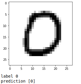
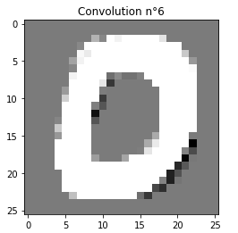
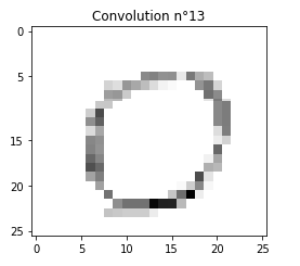
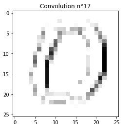
Show me what the network sees
see doc ref: print_convolutions, print_max_poolings
Let’s pick a random image and choose the most significant convolutions
sample_index = 10
show_image(x_test, sample_index)

prediction = model(x_test[sample_index].reshape(1, IMAGE_HEIGHT, IMAGE_WIDTH, 1))

print("label", y_test[sample_index])
print("prediction", tf.math.argmax(prediction, axis=1).numpy())

print_convolutions(model)
print_max_poolings(model)
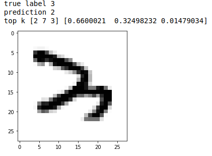
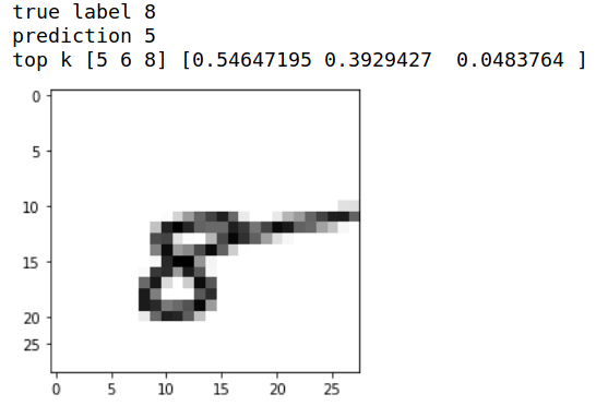
Error analysis
see doc ref: tf.math.top_k
Finally, we perform a short error analysis, to see where the model goes wrong. For this, we picked the model at epoch 5 because it seems to be the less wrong.
epoch = 5
savedModel = tf.saved_model.load("mnist/epoch/{0}".format(epoch))

m = x_test.shape[0]

# calculate prediction
test_predictions = model(x_test.reshape(m, IMAGE_HEIGHT, IMAGE_WIDTH, 1))
error_indices = y_test != np.argmax(test_predictions, axis=1)

error_images = x_test[error_indices]
error_labels = y_test[error_indices]
error_predictions = test_predictions[error_indices]
np.set_printoptions(suppress=True)

for i, error_prediction in enumerate(error_predictions):
  print("index", i)
  print("true label", error_labels[i])
  print("prediction", tf.math.argmax(error_prediction).numpy())

  top3 = tf.math.top_k(error_prediction, 3)
  print("top k", top3.indices.numpy(), top3.values.numpy())

  show_image(error_images, i)
Let’s take a seven misclassified as 2.
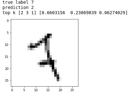
In this case the model is not really good because none of the top 3 predictions are 7 !
We then have two different cases. The next is when the hand wirtten digit is even hard for a human to read. This 3 for exemple:
And this last one, which explains pretty well why CAPTCHAs are so difficult to predict.
Writing this article, I really liked the following sources