Four simple instantiations of ARIMA processes as a cheat sheet
This post is just about simple ARIMA processes, some common notations and functions in time series analysis.
Table of contents
General notations
ARIMA processes can be expressed with a parametric equation:
\[z_t' = \phi_0 + \sum^p_{i=1}\phi_i z'_{t-i} + \epsilon_t + \sum^q_{i=1}\theta_i\epsilon_{t-i}\] \[z_t' = \phi_0 + \phi_1 z'_{t-1} + \phi_2 z'_{t-2} + ... + \phi_p z'_{t-p} + \epsilon_t + \theta_1 \epsilon_{t-1} + \theta_2 \epsilon_{t-2} + ... + \theta_q \epsilon_{t-q}\]where
- \(z_t'\) is the \(z_t\) variable after \(d^{th}\) differentiations
- \(\epsilon_t \sim N(0,1)\) is gaussian white noise with zero mean and unit variance
- \(p,d,q\) are integers
- \(\{ \phi_i \}\) and \(\{ \theta_i \}\) are model parameters, all reals
ARIMA processes can also be expressed with the help of a backward shift operator:
\[\Phi_p(B)(1 - B)^dz_t = \Theta_q(B)\epsilon_t\]where
- \(B\) is the backward shift operator defined as \(Bz_t = z_{t-1}\), and more generally for \(k \in \mathbb{N}^+\)
-
\(\Phi_p\) is a polynomial in \(B\) such as \(\Phi_p(B) = 1 -\phi_1B - \cdots - \phi_pB^p\)
-
and \(\Theta_q\) is a polynomial in \(B\) with \(\Theta_q(B) = 1 + \theta_1B + \cdots + \theta_qB^q\)
Can also be written with the gradient (\(\nabla\)) operator:
\[\Phi_p(B)\nabla^dz_t = \Theta_q(B)\epsilon_t\]Codependencies
A correlation of a variable with itself at different times is known as autocorrelation. When a value \(Z_t\) is correlated with a subsequent value \(Z_{t+h}\) at lag \(h\) then autocovariance function can be expressed as:
\[Cov(Z_t, Z_{t+h}) = \gamma_Z(h) = E[(Z_t - \mu_t)(Z_{t+h} - \mu_{t+h})]\]If a time series model is second-order stationary, which means stationary in both mean and variance, \(\forall t\): \(\mu_t = \mu\) and \(\sigma_t = \sigma\), then:
\[Cov(Z_t, Z_{t+h}) = \gamma_Z(h) = E[(Z_t - \mu)(Z_{t+h} - \mu)]\]Autocorrelation function is defined as:
\[ACF(Z_t, Z_{t+h}) = \rho_Z(h) = { Cov(Z_t, Z_{t+h}) \over \sqrt{ Var(Z_t) Var(Z_{t+h}) } } = { \gamma_Z(h) \over \gamma_Z(0) } = { \gamma_Z(h) \over \sigma^2 }\]The partial autocorrelation function (PACF) at lag \(h\) shows the autocorrelation between \(Z_t\) and \(Z_{t+h}\) after the dependencies of \(Z_t\) on \(Z_{t+1} \cdots Z_{t+h-1}\) have been removed.
It can be shown that the PACF is the correlation between the prediction errors \(Z_t - \hat{Z}_t\) and \(Z_{t+h} - \hat{Z}_{t+h}\):
\[PACF(Z_t, Z_{t+h}) = \alpha_Z(h) = Cor(Z_t - \hat{Z}_t, Z_{t+h}-\hat{Z}_{t+h})\]PACF is sensitive to outliers
Simple zero-mean and unit-variance models
In this section we observe simple zero-mean models, where \(\phi_0\) and \(\theta_0\) are equal to zero. We also take \(\{ \epsilon_t \} \sim N(\mu=0,\sigma^2=1)\). The following table shows the models we’ll analyze.
| Instantiation | ARIMA(p,d,q) |
|---|---|
| Gaussian White Noise | ARIMA(0,0,0) |
| Gaussian Random Walk | ARIMA(0,1,0) |
| First-Order Linear Autoregression | ARIMA(1,0,0) |
| First-Order Moving Average | ARIMA(0,0,1) |
Gaussian White Noise - ARIMA(0,0,0)
A white noise process is the special case of an ARIMA process when \(p= d =q =0\).
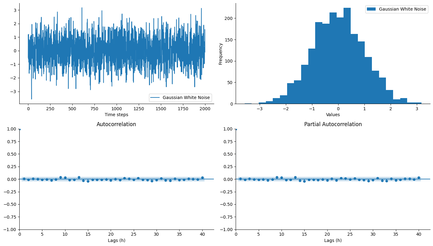
| Parametric Notation | Backward Shift Notation |
|---|---|
| \(z_t = \epsilon_t\) | \(\Phi_0(B)(1 - B)^0 z_t = \Theta_0(B)\epsilon_t\) |
| Autocovariance ACVF | Autocorrelation ACF | Partial Autocorrelation PACF |
|---|---|---|
| \(\gamma_{z}(t + h, t) = \left\{ \begin{array}{ll} 1, & \text{if } h = 0 \\ 0, & \text{if } h \ne 0 \end{array} \right.\) | \(\rho_{z}(h) = \left\{ \begin{array}{ll} 1, & \text{if } h = 0 \\ 0, & \text{if } h \ne 0 \end{array} \right.\) | \(\alpha_{z}(h) = \left\{ \begin{array}{ll} 1, & \text{if } h = 0 \\ 0, & \text{if } h \ne 0 \end{array} \right.\) |
Gaussian Random Walk - ARIMA(0,1,0) - I(1)
A random walk process is the special case of an ARIMA process when \(p=q =0\) and \(d=1\).
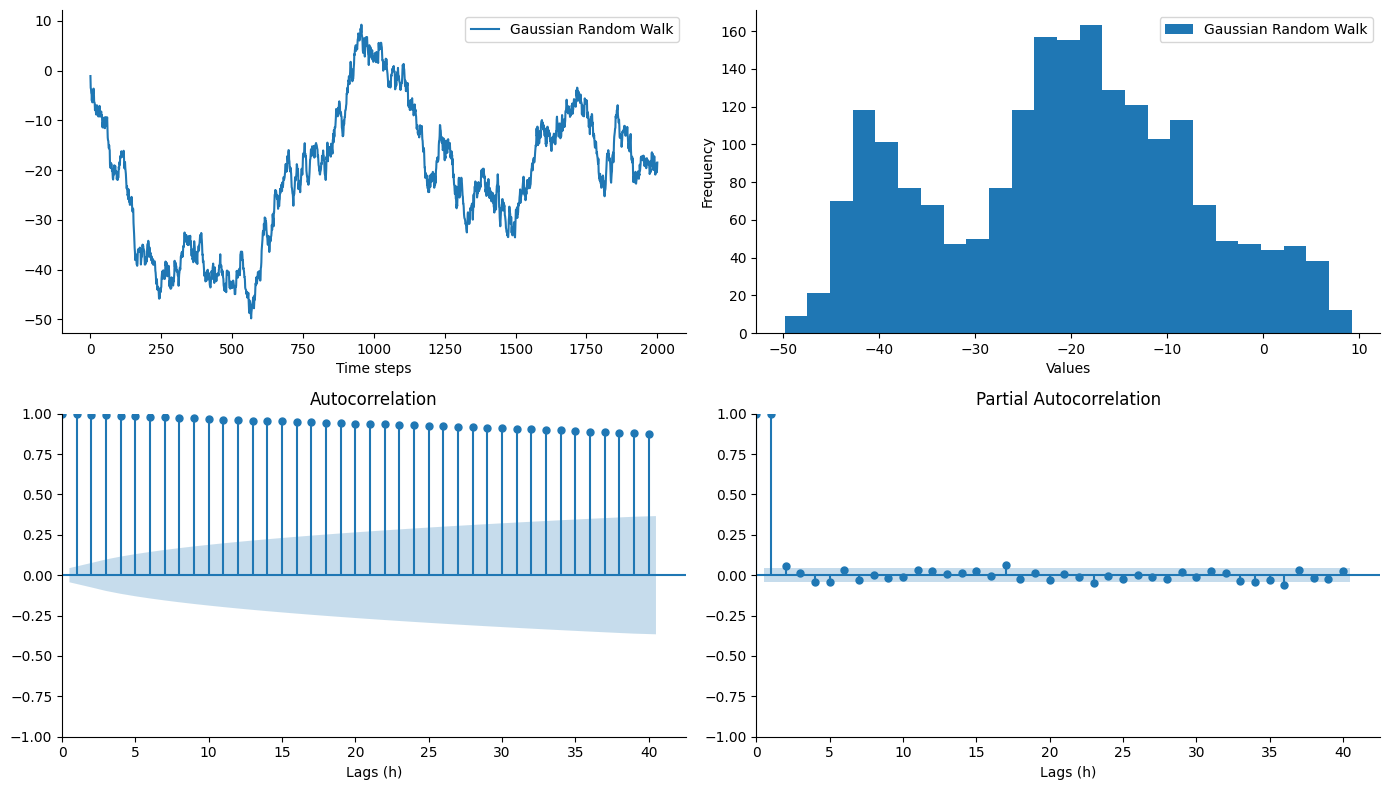
| Parametric Notation | Backward Shift Notation |
|---|---|
| \(z_{t} = z_{t-1} + \epsilon_t\) | \(\Phi_0(B)(1 - B)^1 z_t = \Theta_0(B)\epsilon_t\) |
| Autocovariance ACVF | Autocorrelation ACF | Partial Autocorrelation PACF |
|---|---|---|
| \(\gamma_{z}(t + h, t) = t\) | \(\rho_{z}(h) = 1\) | \(\alpha_z(h) = \left \{ \begin{array}{ll} 1, & \text{if } h \le 1 \\ 0, & \text{if } h \gt 1 \end{array} \right.\) |
First-Order Linear Autoregression - ARIMA(1,0,0) - AR(1)
A first-order autoregressive process is the special case of an ARIMA process when \(p=1\) and \(d=q=0\).
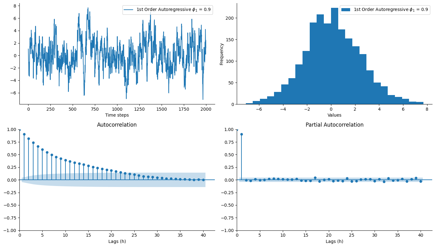
| Parametric Notation | Backward Shift Notation |
|---|---|
| \(z_t = \phi_0 + \sum^p_{i=1} \phi_i z_{t-i} + \epsilon_t\) | \(\Phi_1(B)(1 - B)^0 z_t = \Theta_0(B)\epsilon_t\) |
| \(z_t = \phi_1 z_{t-1} + \epsilon_t\) | \((1 -\phi_1B) z_t = \epsilon_t\) |
| Autocovariance ACVF | Autocorrelation ACF | Partial Autocorrelation PACF |
|---|---|---|
| \(\gamma_{z}(h) = {\phi_1}^h \gamma_{z}(0)\) | \(\rho_{z}(h) = {\phi_1}^{\lvert h \rvert}\) | \(\alpha_z(h) = \left \{ \begin{array}{ll} 1, & \text{if } h = 0 \\ {\phi_1}^2, & \text{if } h = 1 \\ 0, & \text{if } h \gt 1 \end{array} \right.\) |
First-Order Moving Average - ARIMA(0,0,1) - MA(1)
A first-order moving average process is the special case of an ARIMA process when \(p=d=0\) and \(q=1\).
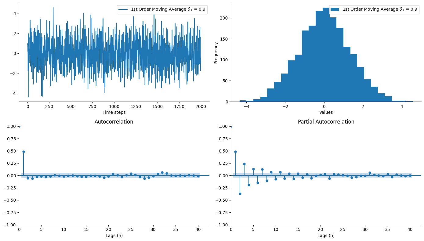
| Parametric Notation | Backward Shift Notation |
|---|---|
| \(z_t = \theta_0 + \sum^q_{i=1} \theta_i \epsilon_{t-i} + \epsilon_t\) | \(\Phi_0(B)(1 - B)^0 z_t = \Theta_1(B)\epsilon_t\) |
| \(z_t = \theta_1 \epsilon_{t-1} + \epsilon_t\) | \(z_t = (1 + \theta_1B)\epsilon_t\) |
| Autocovariance ACVF | Autocorrelation ACF | Partial Autocorrelation PACF |
|---|---|---|
| \(\gamma_{z}(h) = \left\{ \begin{array}{ll} 1 + \theta_1^2, & \text{if } h = 0 \\ \theta_1, & \text{if } h = \pm 1 \\ 0, & \text{if } \lvert h \rvert \gt 1 \end{array} \right.\) | \(\rho_{z}(h) = \left\{ \begin{array}{ll} 1, & \text{if } h = 0 \\ \theta_1^2, & \text{if } h = \pm 1 \\ 0, & \text{if } \lvert h \rvert \gt 1 \end{array} \right.\) | \(\alpha_z(h) = \left \{ \begin{array}{ll} 1, & \text{if } h = 0 \\ { -(- \theta_1)^h \over 1 + \theta_1^2 + \cdots + \theta_1^{2h} }, & \text{if } h \gt 0 \end{array} \right.\) |