How to get collocations with the dunning likelihood ratio?

In this post, I’ll try to explain what a collocation is, how we can retrieve collocations from a text corpus, and how to interpret the results. The main theory explaination of this post is largely inspired (not to say outrageously copied!) by part 5.3.4 of the Foundations of Statistical Natural Language, Manning and Schütze.
After the boring theory, we’ll apply this technic to a french case law dataset. All the code is available in the following git repository judilibre-eda.
Table of content
Definitions
A collocation is an expression consisting of two or more words that correspond to some conventional way of saying things.
As Choueka said:
[A collocation is defined as] a sequence of two or more consecutive words, that has characteristics of a syntactic and semantic unit, and whose exact and unambiguous meaning or connotation cannot be derived directly from the meaning or connotation of its components.
Choueka (1988)
Properties of collocation
More precisly a collocation is a group of words having one or more of the three following properties: non-compositionality, non-substitutability and non-modifiability.
Non-compositionality
Collocations are characterized by limited compositionality in that there is usually an element of meaning added to the combination of the meaning of each part.
Idioms are the most extreme examples of non-compositionality. Idioms like to kick the bucket or to hear it through the grapevine only have an indirect historical relationship to the meanings of the parts of the expression. We are not talking about buckets or grapevines literally when we use these idioms.
Non-substitutability
We cannot substitute near-synonyms for the components of a collocation. For example, we can’t say yellow wine instead of white wine even though yellow is as good a description of the color of white wine as white is (it is kind of a yellowish white).
Non-modifiability
Many collocations cannot be freely modified with additional lexical material or through grammatical transformations. This is especially true for frozen expressions like idioms. For example, we can’t modify frog in to get a frog in one’s throat into to get an ugly frog in one’s throat although usually nouns like frog can be modified by adjectives like ugly. Similarly, going from singular to plural can make an idiom ill-formed, for example in people as poor as church mice.
Types
There a various types of collocations:
- noun phrases, like strong tea and weapons of mass destruction
- phrasal verbs, like to make up, verb particle constructions, important part of the lexicon of English, combination of a main verb and a particle, often correspond to a single lexeme in other languages, often non-adjancent words
- light verbs, like make a decision or do a favor. There is hardly anything about the meaning of make, take or do that would explain why we have to say make a decision instead of take a decision and do a favor instead of make a favor
- stock phrases, like the rich and powerful
- subtle and not-easily-explainable patterns of word usage, like a stiff breeze, or broad daylight
- phraseme or set phrase is a multi word utterance where at least one of whose components is selectionnaly constrained or restricted by linguistic convention such that it is not freely chosen.
- idiomatic phrase or idiom, completely frozen expressions, like proper nouns
- proper nouns, proper names, quite different from lexical collocation but usually included
- saying or a proverb, figure of speech, foxed expression
- terminological expressions, like group of words in technical domains that are often compositional but they may have to be treated consistently for certain NLP tasks such as translation.
Applications in NLP
Collocations are important for a number of applications:
- natural language generation, to make sure that the output sounds natural and mistakes like powerful tea or to take a decision are avoided
- computational lexicography, to automatically identify the important collocations to be listed in a dictionary entry
- word tokenizer/parsing, so that preference can be given to parse with natural collocations
- corpus linguistic research, the study of social phenomena like the reinforcement of cultural stereotypes through language (Stubbs 1996)
Co-occurrence VS Collocation
In linguistics, co-occurences or terms associations are graphemes where words are strongly associated with each other, but do not necessarily occur in a common grammatical unit and with a particular order. In other words, a co-occurrence is an extension of word counting in higher dimensions. The co-presence of more than one word/token within the same contextual window has to be statistically significative.
When it’s proved that there is a semantical or gramatical dependency between two words, we call it collocation. Then, collocation is special case of co-occurrence, or “free phrases”, where all of the members are chosen freely, based exclusively on their meaning and the message that the speaker wishes to communicate.
Co-occurence and semantic field
Co-occurrence can be interpreted as an indicator of semantic proximity. When two words or more have a semantical relationship, co-occurrence notion is at the base of thematic, semantic field and isotopy. It is a more general association of words that are likely to be used in the same context.
In semantic and semiotiquen, isotopy is the redondancy of element in a corpus enabling to understand it. For example, the redondancy of the first person (I), make it easy to understand that the same person is talking. Redondancy of the same semantic field enable us to understand that we are talking about the same theme.
Principal approaches of finding collocations
There are various and complementary ways to look for collocations:
- selection of collocations by frequency
- selection based on mean and variance of the distance between focal word and collocating word
- hypothesis testing
- mutual information
In the remaining parts of this post, we are going to focus on hypothesis testing and more specifically on the likelihood ratio test.
Dunning likelihood collocation score
Likelihood ratios are more appropriate for sparse data than the \(\chi^2\) test. But they also have the advantage that the statistic we are computing, a likelihood ratio, is more interpretable than the \(\chi^2\) statistic.
At the end, the likelihood ratio is simply a number that tells us how much more likely one hypothesis is than the other.
In applying the likelihood ratio test to collocation discovery, we examine the following two alternative explanations for the occurrence frequency of a bigram \(w_1 w_2\) (Dunning 1993)
- First hypothesis is \(H_1 : Pr(w_2 \vert w_1) = p = Pr(w_2 \vert \bar{w_1} )\)
- Second hypothesis is \(H_2 : Pr(w_2 \vert w_1) = p_1 \ne p_2 = Pr(w_2 \vert \bar{w_1} )\)
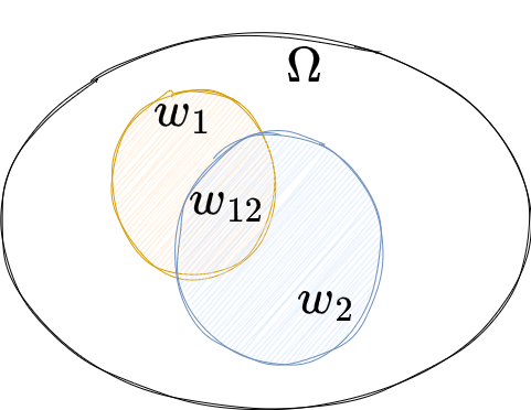
Given \(c_1 = \vert w_1 \vert\), \(c_2 = \vert w_2 \vert\) and \(c_{12} = \vert w_{12} \vert\) are the number of occurences of the corresponding grapheme and \(N = \vert \Omega \vert\) the total number of tokens/words in the corpus, we define the probability of having this two words adjacent, and the opposite probability:
- \(Pr(w_2 \vert w_1) = p_1 = { c_{12} \over c_1 }\),
- \(Pr(w_2 \vert \bar{w_1} ) = p_2 = { c_2 - c_{12} \over N - c_1 }\).
The next table shows the probability of having words \(w_2\) and \(w_1\) adjacent, and the probability of having word \(w_2\) not adjacent to \(w_1\).
| \(Pr(w_2 \vert w_1)\) | \(Pr(w_2 \vert \bar{w_1} )\) | |
|---|---|---|
| \(H_1\) | \(p_1=p={ c_2 \over N }\) | \(p_2=p= { c_2 \over N }\) |
| \(H_2\) | \(p_1={ c_{12} \over c_1 }\) | \(p_2= { c_2 - c_{12} \over N - c_1 }\) |
Following the first hypothesis, the likelihood of observing the data given \(H_1\) is the product of the likelihood of observing \(c_{12}\) words out of \(c_1\) with the likelihood of observing \(c_2 - c_{12}\) words out of \(N - c_1\):
\[L(H_1) = Pr( w_2 \vert w_1, H_1) \times Pr( w_2 \vert \bar{w_1}, H_1)\]We note \(b()\) the probability mass function of the binomial distribution:
\[b(k;n,p) = \binom{n}{k} p^k (1-p)^{n-k}\]So that the likelihood of \(H_1\) can be written:
\[L(H_1) = b(c_{12};c_1,p) \times b(c_2 - c_{12};N - c_1,p)\]Similarly the likelihood of observing the data given \(H_2\) is the product of the likelihood of observing \(c_{12}\) words out of \(c_1\) with the likelihood of observing \(c_2 - c_{12}\) words out of \(N - c_1\):
\[L(H_2) = Pr( w_2 \vert w_1, H_2) \times Pr( w_2 \vert \bar{w_1}, H_2)\] \[L(H_2) = b(c_{12};c_1,p_1) \times b(c_2 - c_{12};N - c_1,p_2)\]The likelihood ratio \(\lambda\) is the quotient of the likelihoods:
\[\lambda = { L(H_1) \over L(H_2) }\]Generally if \(\lambda \gt 1\) the first hypothesis is more likely than the second. For instance, if \(\lambda = 4\) then the \(H_1\) is four times more likely than \(H_2\) to happen. In our case, the first hypothesis is much less likely than the second one. So it is common to take the logarithm of the ratio, with a negative constant before \(-2 log(\lambda)\).
Advantages of likelihood ratio
One advantage of likelihood ratios is that they have a clear intuitive interpretation. They can also be more appropriate for sparse data than the \(\chi^2\) test.
For hypothesis testing, if \(\lambda\) is a likelihood ratio of a particular form, then the quantity \(-2 log(\lambda)\) is \(\chi^2\) distributed when the data sample is large enough. So giving that \(-2 log(\lambda) \sim \chi^2\) we can test the hypothesis \(H_1\) against the alternative hypothesis \(H_2\).
In the next section we are going to apply the likelihood ratio to find collocation in a case law corpus.
Sample use case on Judilibre Open Data
If you are interested in data extraction, you’d like to have a look at the python generated swagger client available here.
The French court of cassation initiated the JUDILIBRE project aimed at the design and in-house development of a search engine in the corpus of case law, making it available to the public.
After extracting an arbitrary part of the corpus through the search engine API, I persisted the results in a json line file.
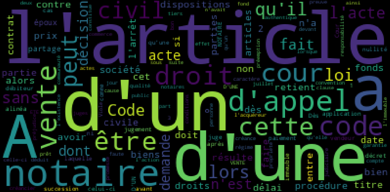
Word Cloud
Just a quick look at a word cloud illustration of the dataset:
Bigram collocation
The method collocation_2 enable us to find collocations and ordered them following the negative log likelihood score:
collocation_2(judilibre_text, method="llr", stop_words=stop_words)
{"cour d'appel": 14779.656345618061,
 'code civil': 9034.437842527477,
 'dès lors': 8061.607047568378,
 'bon droit': 2470.063562327007,
 'procédure civile': 2074.7855327925286,
 'peut être': 1936.8836188208438,
 'doit être': 1856.4831975258871,
 "d'un immeuble": 1694.5615662280786,
 'chose jugée': 1512.3425659159825,
 'après avoir': 1478.3002163179476,
 'condition suspensive': 1253.7851148695208,
 'rédaction antérieure': 1221.519857102709,
 'base légale': 1133.1024031677157,
 'sous seing': 1120.8378898578583,
 'seing privé': 1114.6228341225883,
 "d'autre part": 1037.4683304932462,
 "qu'une cour": 990.3205509155646,
 "cassation l'arrêt": 977.635114391793,
 "l'acte authentique": 969.402554409081,
 "d'un acte": 947.6827965402367}
The bigram cour d’appel is more than 14000 times more likely under the \(H_2\) hypothesis (d’appel is more likely to follow cour) than its base rate of occurrence would suggest.
Pointwise mutual information
It may be interesting to look at the collocations ranked by the pointwise mutual information, another hypothesis test method:
collocation_2(judilibre_text, method="pmi", stop_words=stop_words)
{'bonnes moeurs': 17.259674311869706,
 "d'échelle mobile": 17.259674311869706,
 "donneur d'aval": 17.259674311869706,
 'maniere fantaisiste': 17.259674311869706,
 "pétition d'hérédité": 17.259674311869706,
 'simulations chiffrées': 17.259674311869706,
 'trimestre echu': 17.259674311869706,
 'viciait fondamentalement': 17.259674311869706,
 '1035 1036': 16.674711811148548,
 '13-18 383': 16.674711811148548,
 '757 758-6': 16.674711811148548,
 'associations syndicales': 16.674711811148548,
 'coemprunteurs souscrivent': 16.674711811148548,
 'collectivités territoriales': 16.674711811148548,
 'dissimulée derrière': 16.674711811148548,
 "désirant l'acquérir": 16.674711811148548,
 'endettement croissant': 16.674711811148548,
 'huis clos': 16.674711811148548,
 'mètre carré': 16.674711811148548,
 'potentiellement significatives': 16.674711811148548}
P-value
If we want a more detailed output we can use the detailed_collocation_2 function:
| \(w_1\) | \(\vert w_1 \vert\) | \(w_2\) | \(\vert w_2 \vert\) | score | p-value | |
|---|---|---|---|---|---|---|
| 0 | cour | 948 | d’appel | 1230 | 14779.7 | 0 |
| 1 | code | 1051 | civil | 830 | 9034.44 | 0 |
| 2 | dès | 477 | lors | 773 | 8061.61 | 0 |
| 3 | bon | 205 | droit | 972 | 2470.06 | 0 |
| 4 | procédure | 496 | civile | 371 | 2074.79 | 0 |
| 5 | peut | 817 | être | 952 | 1936.88 | 0 |
| 6 | doit | 368 | être | 952 | 1856.48 | 0 |
| 7 | d’un | 1879 | immeuble | 261 | 1694.56 | 0 |
| 8 | chose | 157 | jugée | 110 | 1512.34 | 0 |
| 9 | après | 296 | avoir | 326 | 1478.3 | 0 |
| 10 | condition | 175 | suspensive | 73 | 1253.79 | 0 |
| 11 | rédaction | 189 | antérieure | 132 | 1221.52 | 0 |
| 12 | base | 99 | légale | 156 | 1133.1 | 0 |
| 13 | sous | 247 | seing | 67 | 1120.84 | 0 |
| 14 | seing | 67 | privé | 84 | 1114.62 | 0 |
| 15 | d’autre | 69 | part | 210 | 1037.47 | 0 |
| 16 | qu’une | 302 | cour | 948 | 990.321 | 0 |
| 17 | cassation | 186 | l’arrêt | 329 | 977.635 | 0 |
| 18 | l’acte | 647 | authentique | 227 | 969.403 | 0 |
| 19 | d’un | 1879 | acte | 538 | 947.683 | 0 |
| 20 | justifie | 38 | légalement | 139 | 917.195 | 0 |
| 21 | viole | 89 | l’article | 1901 | 914.622 | 0 |
| 22 | société | 411 | civile | 371 | 866.908 | 0 |
| 23 | officier | 63 | public | 217 | 851.046 | 0 |
| 24 | acte | 538 | authentique | 227 | 786.687 | 0 |
| 25 | cet | 322 | acte | 538 | 766.902 | 0 |
| 26 | cet | 322 | officier | 63 | 760.165 | 0 |
| 27 | régime | 191 | matrimonial | 54 | 736.566 | 0 |
| 28 | bonne | 48 | foi | 86 | 734.162 | 0 |
| 29 | sécurité | 49 | sociale | 63 | 732.558 | 0 |
For example, we can look up the value of sécurité sociale in the table and reject \(H_1\) for this bigram on a confidence level of 5% since the critical value for one degree of freedom is 7.88.
Sources
- Foundations of Statistical Natural Language, Manning and Schütze
- Word association norms, mutual information, and lexicography
- NLTK documentation on collocations
- Wikipedia definition of Collocation
- Wikipedia definition of Co-occurrence
- Pointwise Mutual information
- Mutual information
- Information theory