How to statistically test the residuals from forecasted data?

In this post I will test the estimated noise sequence from the difference between the forecast and the actual time series. Taking the 2020’s electricity consumption in France and comparing it to the forecasts. First I’m going to test the raw residuals coming from the difference between the forecast and the consumption. In a second part I’ll fit a SARIMA model to the preceding residuals to further perform the same tests and compare them.
Table of contents
- Electric energy consumption in France
- J-1 Forecast Evaluation
- SARIMA Residuals J-1 Forecast Evaluation
- Final Comparison
- Sources
First, let’s make a brief scan of the dataset, mostly by visual checking, without getting to much into the details.
Electric energy consumption in France
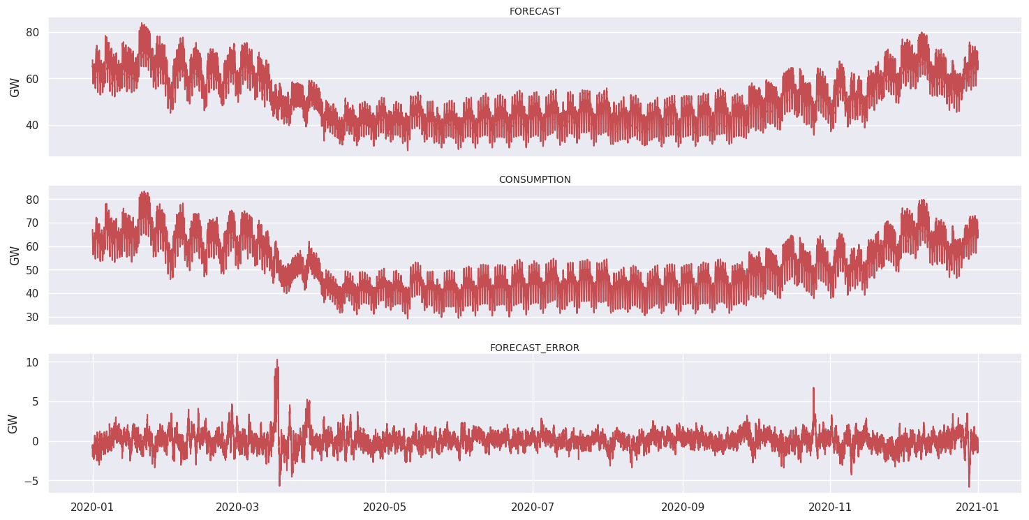
Let’s see the shape of the electricity consumption in France for year 2020. We also plot the forecast and the forecast error. The forecast error is the consumption minus the forecast.
Data integrity
Firstly I performed a brief sanity check. Since the dataset sample rate is initially 15 minutes but only half hour data are provided, I removed the null values. Then I checked that the time steps are constant and continue over time.
Behavior shifts
Looking at the time serie of the consumption of electricity, we can easily see two different regimes. One in winter with a high consumption of electric energy and another in summer when people tend to consume less electricity (in France at least).
Extreme values
No extreme values seem to be present neither in the forecast nor in the prediction. However, the forecast error do seem to have a few extreme values.
There are about 70 values where the forecast error is greater than 5 GigaWatts in absolute value:
\[\lvert {FORECAST}\_{ERROR} \rvert > 5 GW\]Note that 5 GigaWatts is a quite arbitrary value. Giving that 1 MegaWatts is equivalent to the consumption of about 600 homes, then 5GW would be of about 3 millions homes, which is quite a number in comparison with the France population, which has about 30 millions homes, knowing than more that one third of the total electric power consumption is consumed by private homes.
First lock down due to Covid
The spread of the coronavirus among the population leads to a national lock down in France. Looking at the time series, the unusual situation cause a higher variance during a few days. As a result, forecast the electricity consumption one day ahead had to be trickier than usual and over or underestimations of the consumption happened. For instance, the 17th of March might be the day with the higher forecast error, with an error peak at almost 10 GigaWatts.
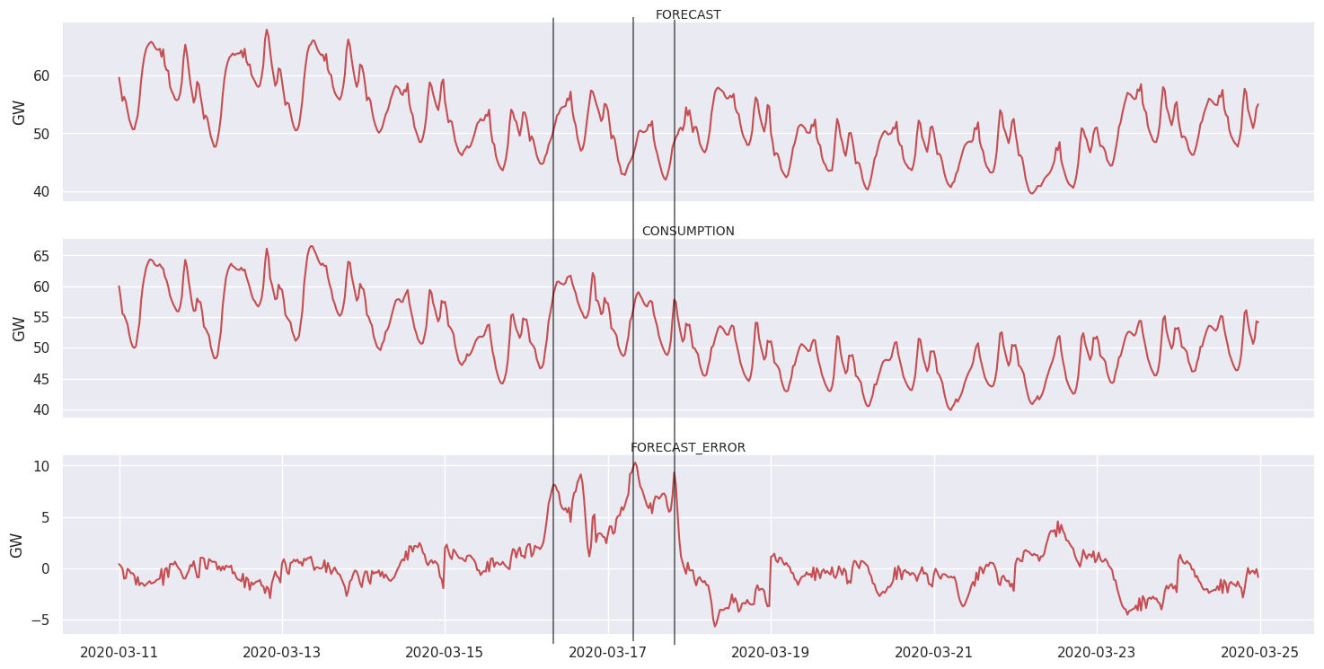
| Thursday, March 12 | Childcare centers are closed, as well as elementary schools and universities |
| Saturday, March 14 | Third and last stage of the crisis plan announced by the prime minister |
| Tuesday, March 17 | Lock down, movement restriction in all European Union, frontiers of the Schengen Area are closed |
Second lock down
During the second lock down, the perturbations in the forecast error were less important. Sunday 25th of October was the day is the higher forecast error on this period. The error peaked at 6 GW and lasted for 1/2 hour, underestimating the consumption.
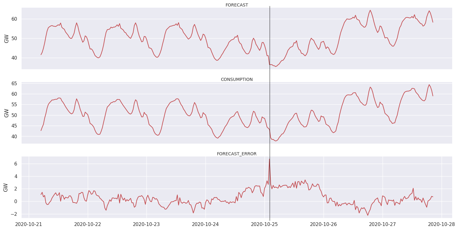
| Saturday, October 17 | Mandatory curfew in certain regions for at least 4 weeks (Ile de France, and eight other cities. Meetings are limited to 6 people. |
| Thursday, October 22 | Curfew extension to 38 new french departements, in addition to the 16 departements already curfewed |
| Friday, October 30 | Generalized lock down. Mandatory lock down of non-essential stores. Movement restriction. Unlike the first lock down childcare centers and schools stay opened |
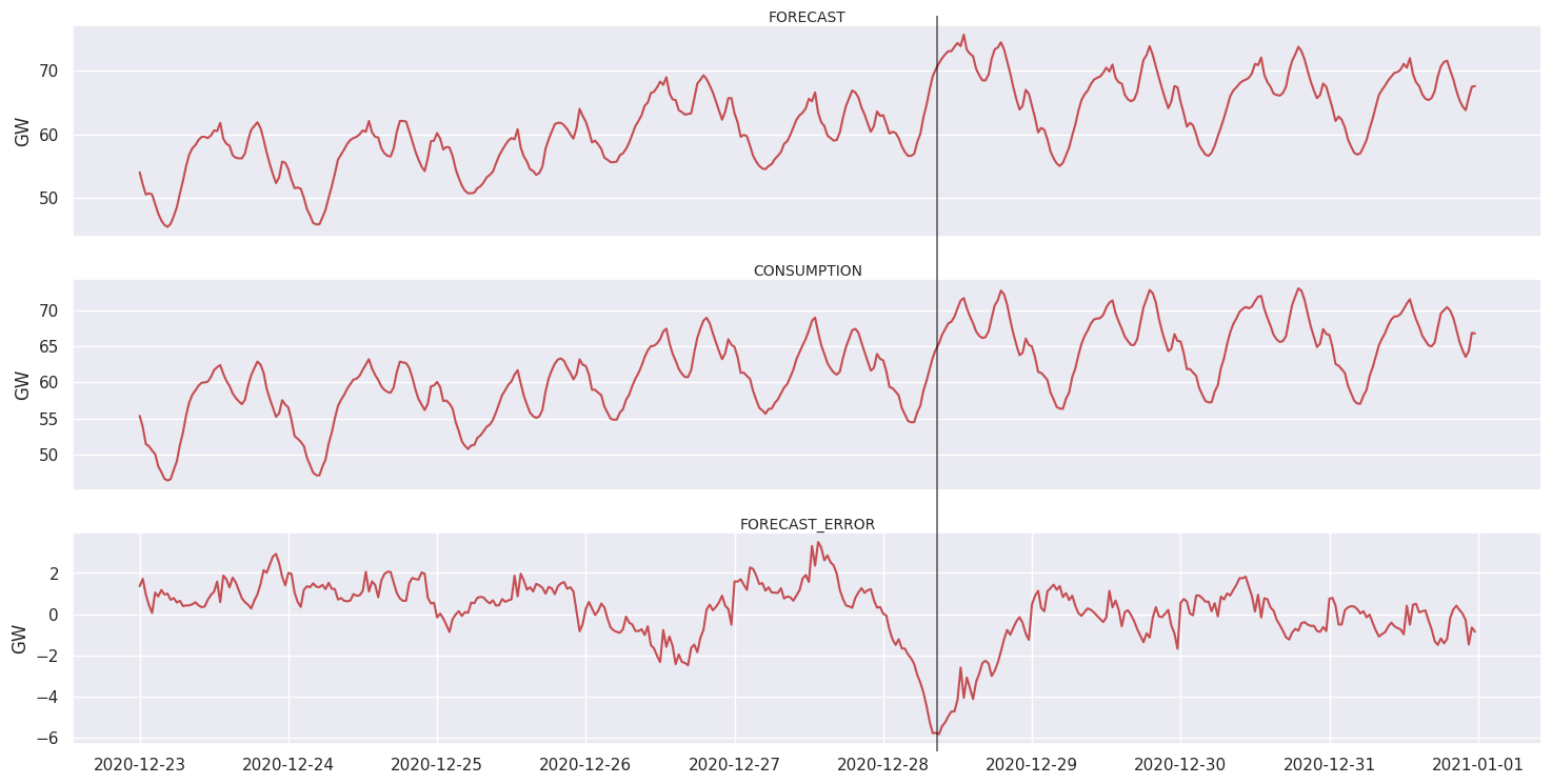
Christmas 2020
As for christams 2020, there is an unusual error in the forecast. This time it’s an overestimation of the consumption.
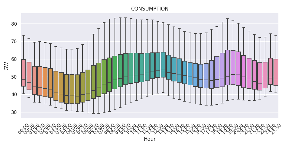
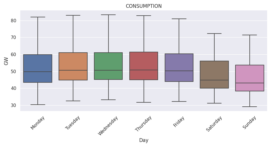
Seasonalities
As one can expect, there might be at least 2 kind of seasonality in this time series: daily and weekly.
J-1 Forecast Evaluation
The residuals are the prediction errors
\[w_t = {Consumption}_t - {Forecast}_t= x_t - \hat{x_t}\]If \(w_t\) is positive, electric power consumption was greater than expected, otherwise it was underestimated.
Basic informations
| count | mean | std | variance | skewness | kurtosis | |
|---|---|---|---|---|---|---|
| PREVISION_ERROR | 17568 | 0.115271 | 1.11063 | 1.23351 | 0.88854 | 7.09978 |
| count | min | 25% | median | 75% | max | |
|---|---|---|---|---|---|---|
| PREVISION_ERROR | 17568 | -5.819 | -0.519 | 0.102 | 0.695 | 10.299 |
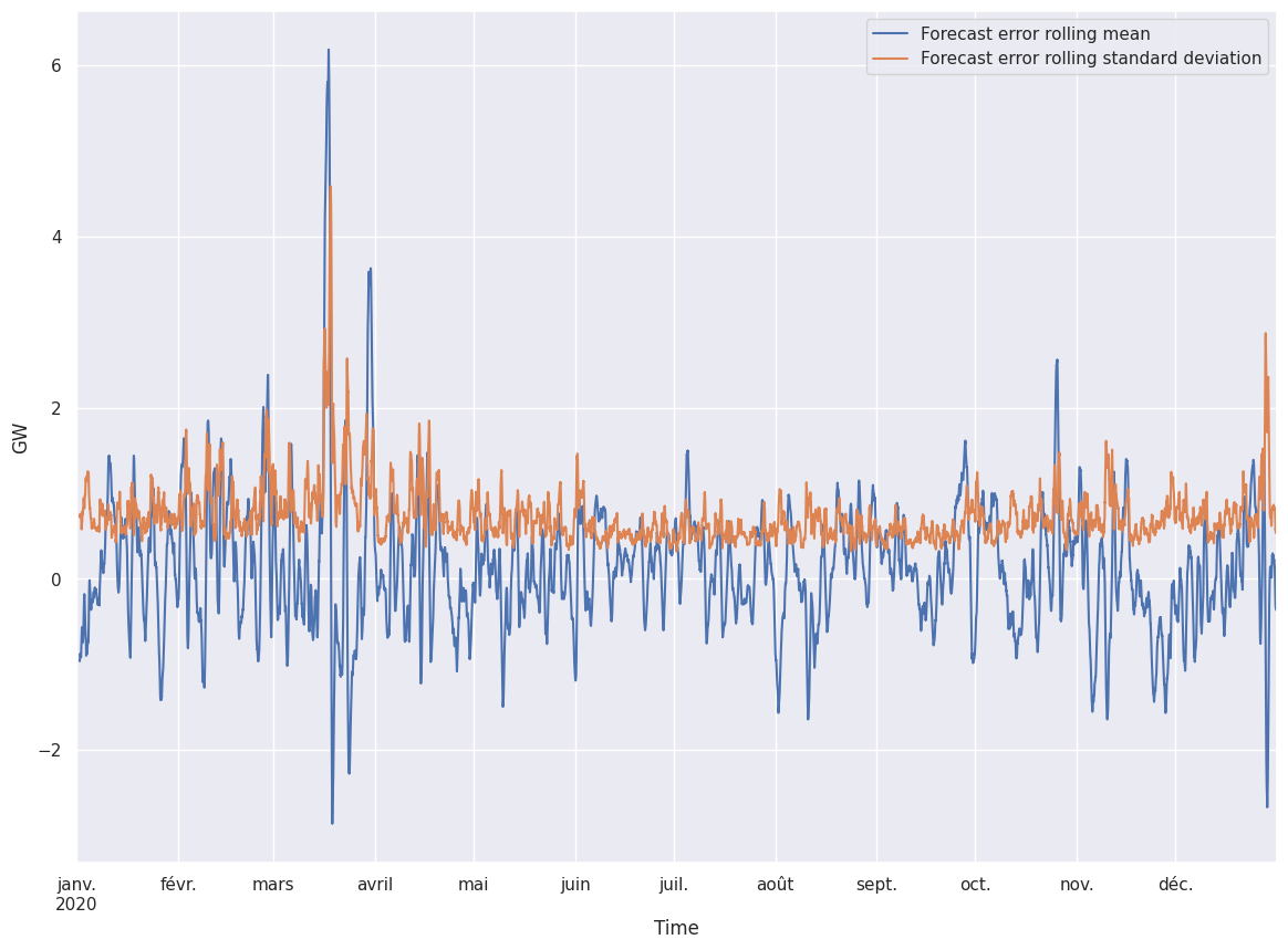
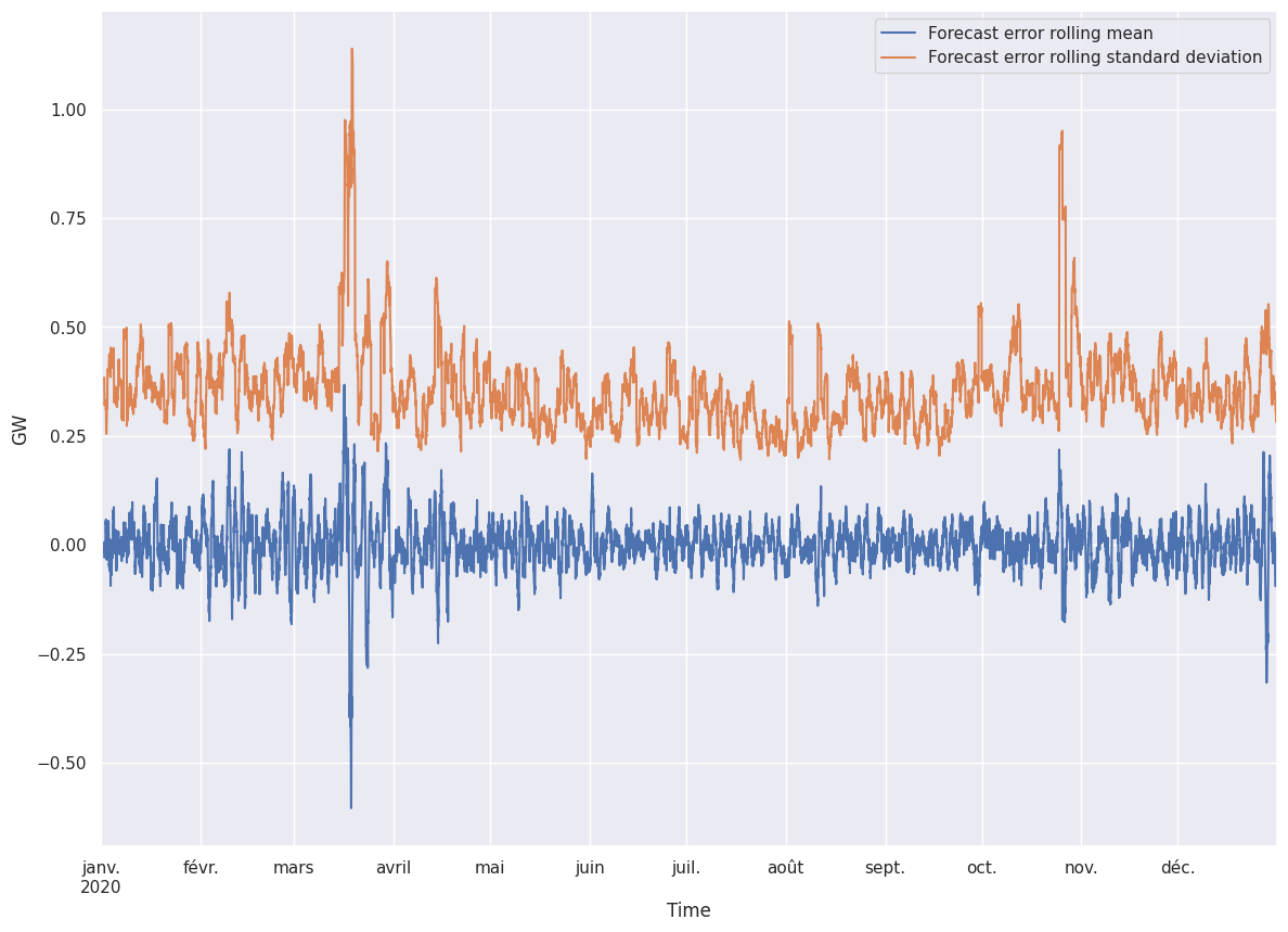
24-hours window rolling statistics
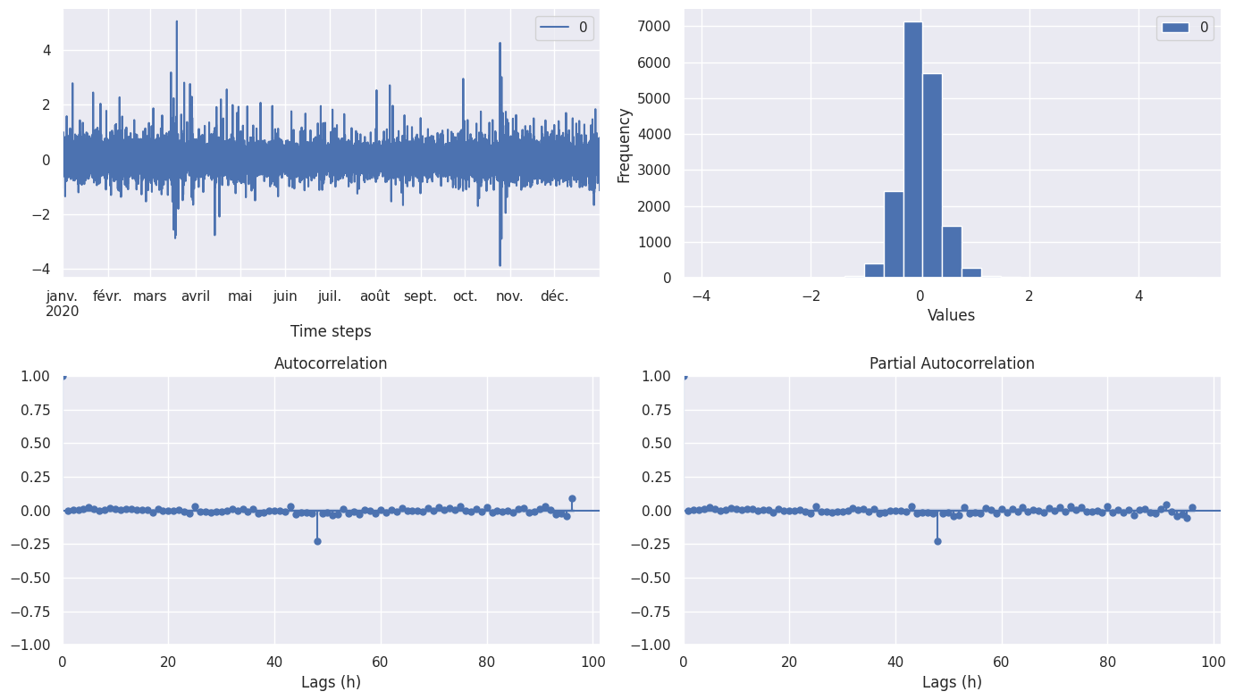
Autocorrelation tests
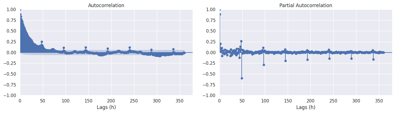
Correlogram
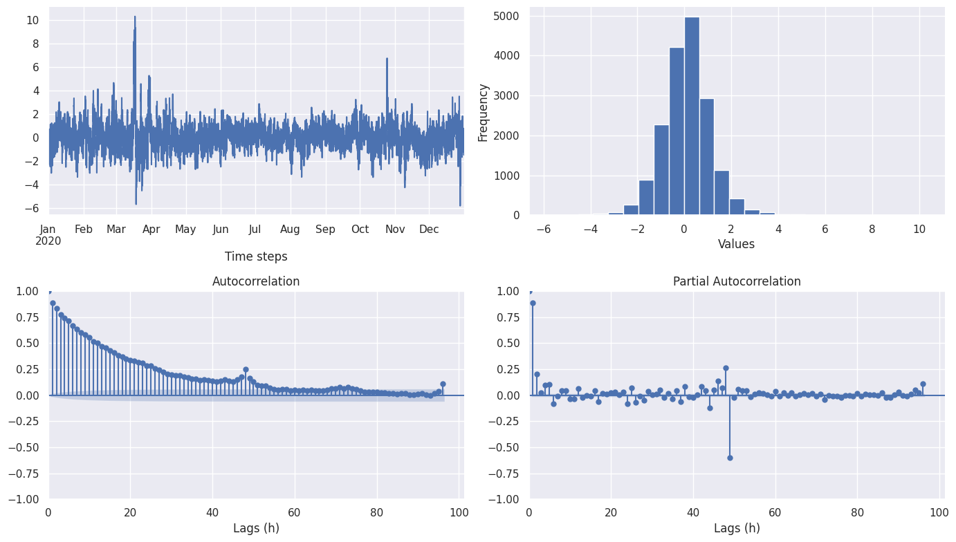
From the correlograms we can see that:
- Autocorrelation slowly decay
- Looking at the PACF, it would be possible to fit and AR(1) or AR(2) model
- Peaks are present at around 24 hours (\(48 \times {1 \over 2}\) hours), this shows the presence of a seasonal process every 24 hours
As we we test the randomness of residuals assuming they should be white noise, the confidence intervals of ACF values are at 2 standard errors around 0.
Looking at a correlogram with a maximum lag at more than a week, it seems that the main seasonal effect is at 24 hour interval. Indeed the 24 hour peaks decay every 24h, and no 7 days seasonal effect seems to come out.
Ljung-Box test
Ljung-Box test is a portmanteau test for testing the autocorrelation in either raw data or model residuals.
| Lags | \(Q_{LB}\) statistic | p-value |
|---|---|---|
| 96 | 142969 | 0 |
| 144 | 143366 | 0 |
Since the test statistic is high 143366 and the p-value is \(<<\) 0.05 we reject the iid hypothesis at level 0.05. It suggests that the sample autocorrelations are too large to be a sample from an iid sequence. We reject the null hypothesis of the test and conclude that the residuals are not independent.
McLeod-Li test
McLeod-Li test is a also a portmanteau test similar to Ljung-Box test. Since p-values for lags [0,…,144] are \(<<\) 0.05 we reject the iid hypothesis at level 0.05. We reject the null hypothesis of the test and conclude once again that the residuals are not independent.
Independence tests
Turning Point Test
Turning Point test is a test of statistical independence of a data series. It can detect cyclic trends. Under the hood, the turning point test compares the number of turning points present in the series with the number of turning points expected to be present in an i.i.d. series.
| \(T\) statistic | p-value | n | \(\mu\) | \(\sigma\) |
|---|---|---|---|---|
| -41.5094 | 0 | 17558 | 11704 | 55.8668 |
Since \(T - \mu\) is way below zero, it indicates that there might be a positive correlation between neighboring observations. The p-value is \(<<\) 0.05, we reject the null hypothesis that the data series is i.i.d., then the data serie probably has a remaining periodic trend.
Rank Test
The rank test is useful for detecting linear trends in data series by comparing the number of increasing pairs in the series with the number expected in an i.i.d. series.
| \(P\) statistic | p-value | pairs | n | \(\mu\) | \(\sigma\) |
|---|---|---|---|---|---|
| -4.56648 | 4.95979e-06 | 7.52957e+07 | 17558 | 7.70665e+07 | 387775 |
Since the \(P - \mu\) is large negative -7e+07, it indicates the presence of an decreasing trend in the data. The assumption that \({w_t}\) is a sample from an iid sequence is therefore rejected at level 0.05, giving the p-value is \(<<\) 0.05.
Stationarity tests
KPSS Test
| KPSS test Statistic | p-Value | # Lags Used | Critical Value (10%) | Critical Value (5%) | Critical Value (2.5%) | Critical Value (1%) |
|---|---|---|---|---|---|---|
| 0.246049 | 0.1 | 144 | 0.347 | 0.463 | 0.574 | 0.739 |
The null hypothesis \(H_0\) is that the data is stationary around a determinist trend. Since \(p>0.05\), we cannot reject the null hypothesis, thus the time series has no unit root, and seems stationary.
Augmented Dickey-Fuller Test
| ADF Test Statistic | p-Value | # Lags Used | # Observations Used | Critical Value (1%) | Critical Value (5%) | Critical Value (10%) |
|---|---|---|---|---|---|---|
| -10.0775 | 1.21258e-17 | 144 | 17423 | -3.43073 | -2.86171 | -2.56686 |
Since \(p<0.05\) we can reject the null hypothesis that the time series has a unit root. Then the alternative hypothesis \(H_a\) the time series hasn’t a unit root, seems to be stationary.
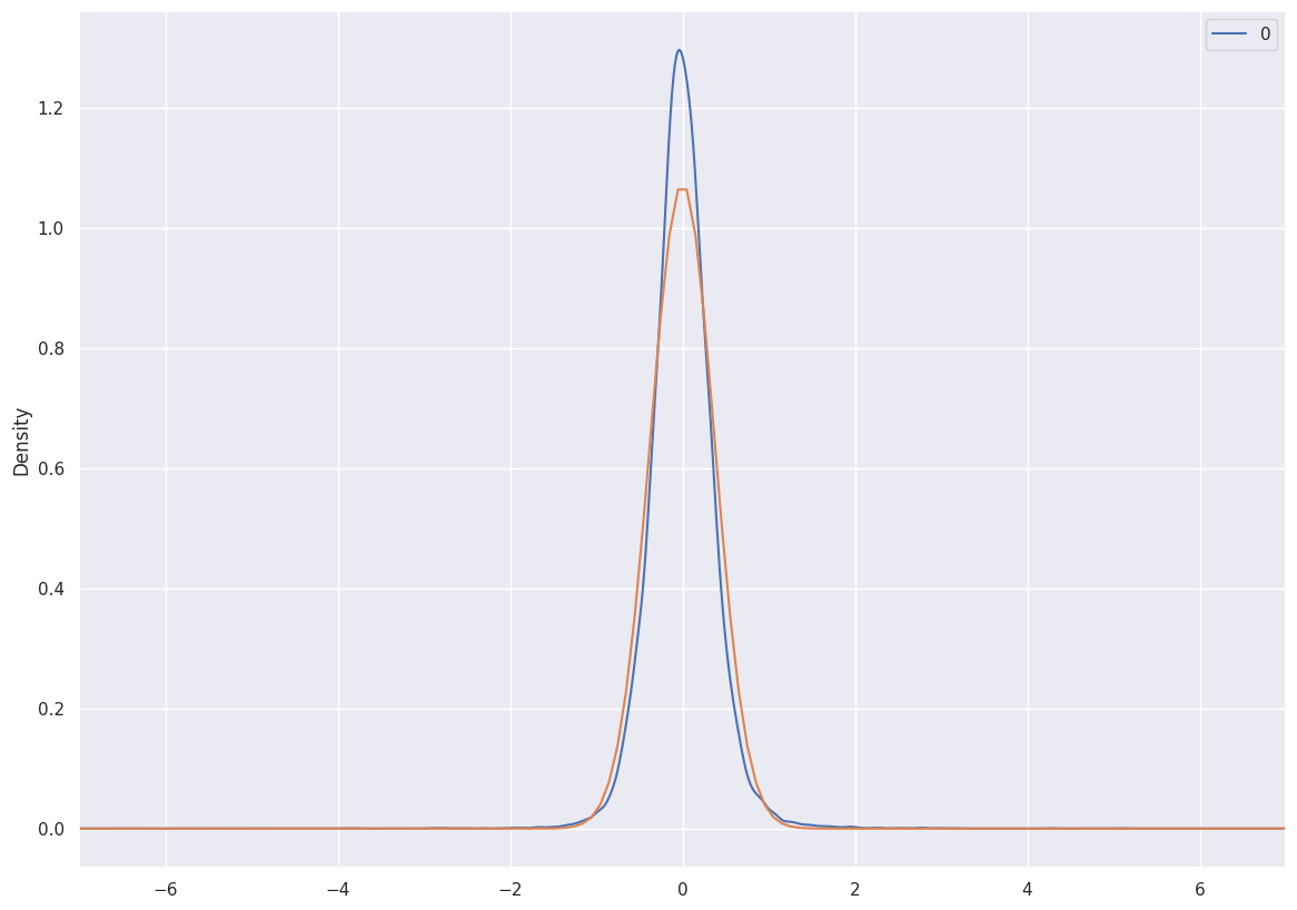
Normality tests
Here we plot the sample distribution of the forecast error in blue, and the ideal gaussian density distribution in orange.
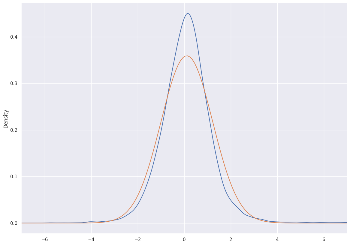
The sample distribution calculated with kernel density estimation seems higher, and seems to have a fatter tail than the gaussian, maybe due to outliers.
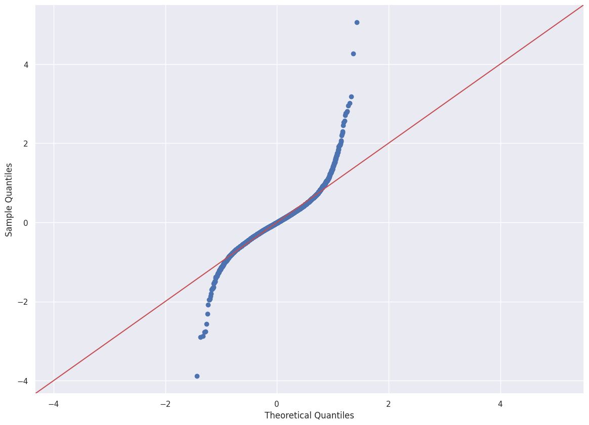
Q-Q plot
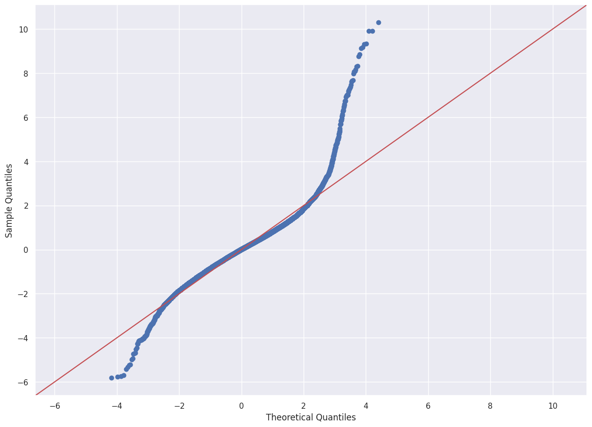
Both the ends of the Q-Q plot deviate from the straight line and its center follows a straight line. Kurtosis is 8, confirm that the tail is larger than one drawn from a normal distribution.
Jarque-Bera Tests
Since sample size is quite large (> 10000), we can use the Jarque-Bera test.
| J-Q Test Statistic | p-value |
|---|---|
| 39184.568 | 0.0 |
The test statistic is 39184 and the corresponding p-value is \(<<\) 0.05. Since this p-value is less than 0.05, we reject the null hypothesis. This data skewness and kurtosis is significantly different from a normal distribution.
SARIMA Residuals J-1 Forecast Evaluation
\[\Phi_p(L) \Phi_P(L^m) (1-L)^d (1 - L^m)^D X_t = \Theta_q(L) \Theta_Q(L^m) \epsilon_t\]- (p, d, q): order of the model for the autoregressive, differences, moving average components
- (P, D, Q, m): order of the seasonal component of the model for the
Daily data with periodicity of 24h, so m = 48 in our case, and we take the following parameters:
- order: (p=2, d=0, q=3),
- seasonal order: (P=1, D=0, Q=0, m=48)
For some simple ARIMA models see my previous post Four simple instantiations of ARIMA processes as a cheat sheet
Basic informations
| count | mean | std | variance | skewness | kurtosis |
|---|---|---|---|---|---|
| 17568 | -4.26557e-06 | 0.371329 | 0.137885 | 0.491632 | 8.19931 |
The mean of the SARIMA residuals are closer than 0, and the variance is smaller than the other residuals.
| count | min | 25% | median | 75% | max |
|---|---|---|---|---|---|
| 17568 | -3.8873 | -0.209651 | -0.00853736 | 0.203478 | 5.05434 |
24-hours window rolling statistics
Autocorrelation tests
Correlogram
The correlogram looks like a random noise one except at time lag 49, where it might still remain a seasonal effect.
Ljung-Box test
| Lags | \(Q_{LB}\) statistic | p-value |
|---|---|---|
| 96 | 1464.91 | 1.4445e-243 |
| 144 | 1874.97 | 9.32924e-299 |
We still reject the null hypothesis of the test and conclude that the residuals are not independent.
McLeod-Li test
The p-values for lags [0,…,144] are still way lower than 0.05. We reject the null hypothesis of the test and conclude once again that the residuals are not independent.
Independence tests
Turning Point Test
| \(T\) statistic | p-value | n | \(\mu\) | \(\sigma\) |
|---|---|---|---|---|
| 0.829117 | 0.407038 | 17568 | 11710.7 | 55.8827 |
The p-value is greater than 0.05, we cannot reject the null hypothesis that the time series is i.i.d.. Unlike the precedent residuals, the data points seem much less dependent.
Rank Test
| \(P\) statistic | p-value | pairs | n | \(\mu\) | \(\sigma\) |
|---|---|---|---|---|---|
| -0.0587056 | 0.953187 | 7.71315e+07 | 17568 | 7.71543e+07 | 388106 |
The p-value is 0.95, greater than 0.05, we cannot reject the null hypothesis that the time series is a sample from an iid sequence. Unlike the precedent residuals, the data points seem much less dependent.
Stationarity tests
More or less the same results as for the previous residuals.
KPSS Test
| KPSS test Statistic | p-Value | # Lags Used | Critical Value (10%) | Critical Value (5%) | Critical Value (2.5%) | Critical Value (1%) |
|---|---|---|---|---|---|---|
| 0.0527507 | 0.1 | 144 | 0.347 | 0.463 | 0.574 | 0.739 |
Augmented Dickey-Fuller Test
| ADF Test Statistic | p-Value | # Lags Used | # Observations Used | Critical Value (1%) | Critical Value (5%) | Critical Value (10%) |
|---|---|---|---|---|---|---|
| -14.8331 | 1.88616e-27 | 144 | 17423 | -3.43073 | -2.86171 | -2.56686 |
Normality tests
SARIMA distribution seems more concentrated around the mean. Still higher than the gaussian distribution.
Q-Q plot
The Q-Q plot is quite similar.
Jarque-Bera Tests
| J-Q Test Statistic | p-value |
|---|---|
| 49886.86 | 0.0 |
A value higher than the previous one confirm that the distribution is more concentrated around the mean.
Final Comparison
| Residuals | SARIMA Residuals | Comment | |
|---|---|---|---|
| Mean | 0.115271 | -4.26557e-06 | More centered |
| Standard Deviation | 1.11063 | 0.371329 | |
| Skewness | 0.88854 | 0.491632 | Less right skewed |
| Kurtosis | 7.09978 | 8.19931 | Thinner density distribution |
| Min | -5.819 | -3.8873 | |
| Max | 10.299 | 5.05434 | |
| Median | 0.102 | -0.008537 | |
| Ljung-Box Test | 143366 (0) | 1874.97 (0) | Still not independant |
| McLeod-Li test | NA (0) | NA (0) | Still not independant |
| Turning Point Test | 41.5094 (0) | 0.8291 (0.4070) | Now independent |
| Rank Test | -4.56648 (4.96e-06) | -0.0587 (0.9532) | Now independent |
| KPSS Test | 0.246049 (0.1) | 0.0527507 (0.1) | Still stationary |
| ADF Test | -10.0775 (1.21e-17) | -14.8331 (1.89e-27) | Still stationary |
| Jarque-Bera Test | 39184 (0.0) | 49886 (0.0) | Still not normal |