Coronavirus prediction based on current data
It is unlikely that the number of cases of Covid-19 reported in this blog post accurately represents the actual number of people infected by the novel coronavirus. There are various reasons to that.
First, despite the fact that several countries publish total number of tests performed, there is no centralized database of COVID-19 testing.
Second, countries have different testing strategies, while South Korea seems to test a lot, some Western countries like France or the US seem to have quiet a low testing rate per habitant.
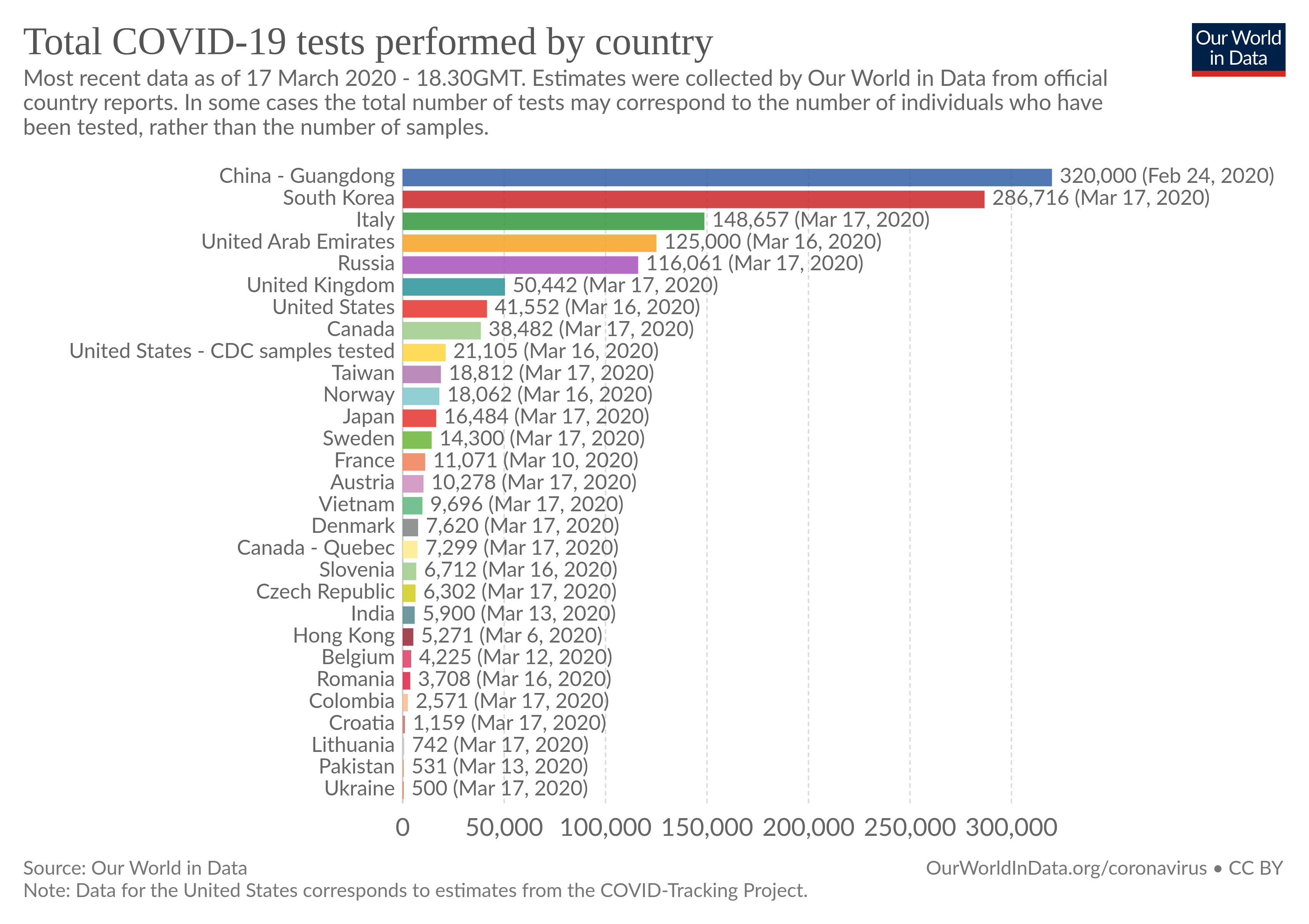
Why testing is so important ? Because we would like to know how many people are currently infected. As the rate of testing increases, the potential difference between the current cases and the confirmed cases decreases.
Third, there are several reasons why someone infected with COVID-19 may produce a false-negative result when tested:
- early stage of the disease with low viral load might be hard to detect
- when no major respiratory symptoms, there could be too little virus quantity in the patient’s throat and nose
- problem with sample collection, handling or shipping of samples and test materials
What we know for sure, with little error, is the number of confirmed cases. That’s the data will be focus on.
You can find the entire notebook at this link.
Prediction with a Sigmoid function
Here I perform a basic regression of a sigmoid function to the data. Here is the form of the function
I also tried with tanh function but I didn’t notice a major difference. So, I’ll stick with the sigmoid in further analysis.
The data comes from the Johns Hopkins University, and this specific repository CSSEGISandData. In this section, I only extract the confirmed cases.
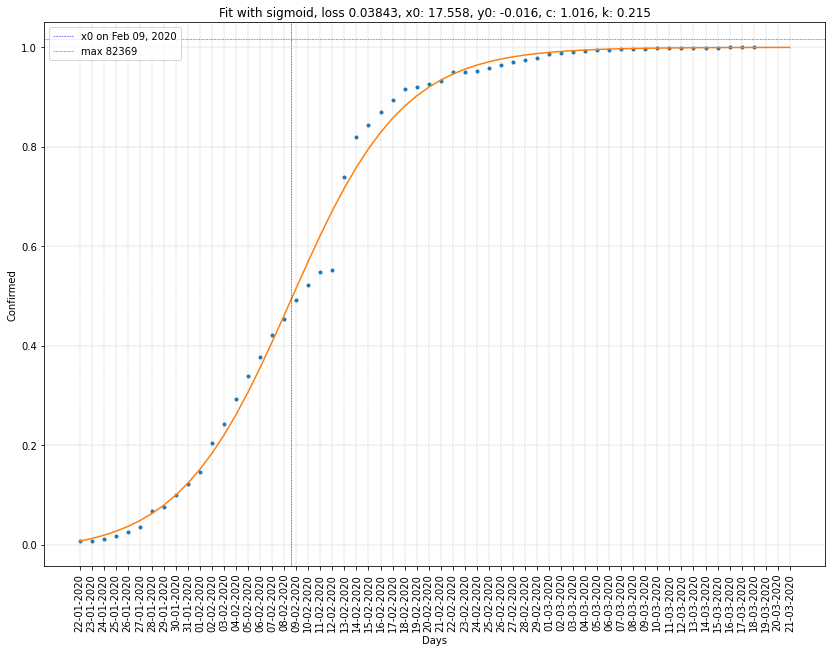
China regression on cumulative confirmed cases
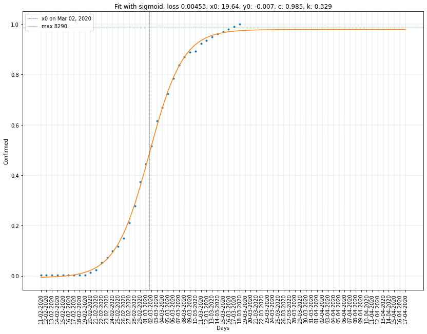
South Korea regression on cumulative confirmed cases
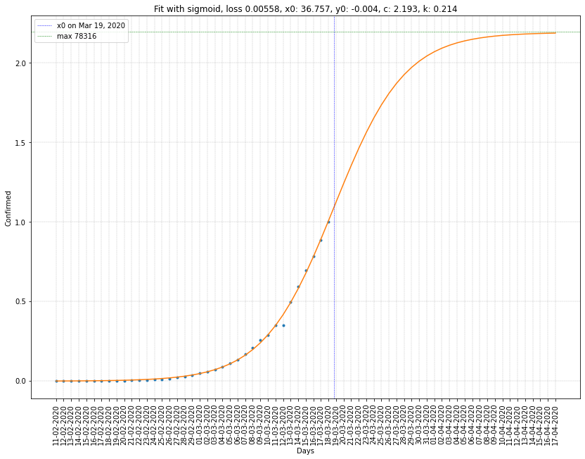
Italy regression on cumulative confirmed cases
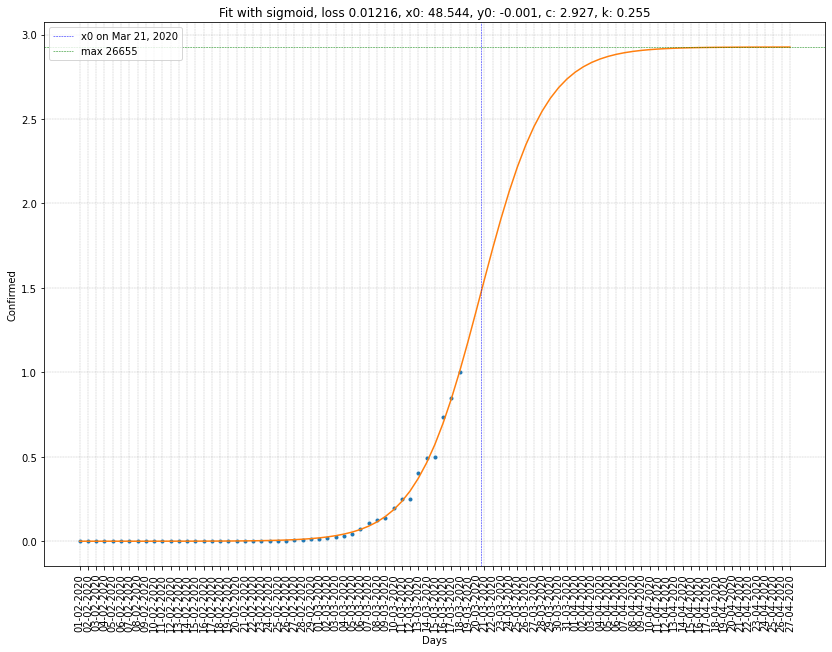
France regression on cumulative confirmed cases
Sigmoid regression summary
I compiled theses numbers in the following table. I omit the parameter \(y_0\) as it is, as expected, very close to 0. However, I should have constrained \(y_0\) to be greater or equal than zero.
- \(x_0\) represents the point of inflexion. Geometrically speaking, the intersection between the curve and the vertical line of abscissa \(x_0\) is a point of symmetry.
- \(c\) represents the height of the curve. I also add the max confirmed cases which came by multipling \(c\) with the current number of cumulative confirmed cases.
- \(k\) represents the steepness. The greater it is, the steeper the curve is.
| Country | \(x_0\) | \(c\) and (max) | \(k\) | loss |
|---|---|---|---|---|
| China | 09/02/2020 | 1.016 (82239) | 0.215 | 0.034 |
| South Korea | 02/03/2020 | 0.985 (8290) | 0.329 | 0.0045 |
| Italy | 19/03/2020 | 2.193 (78316) | 0.214 | 0.0056 |
| France | 21/03/2020 | 2.927 (26655) | 0.255 | 0.0122 |
We have two categories of countries here, the ones where the epidemic passed and the others.
- The firsts have \(x_0\) in the past and \(c\) close to 1. Here again, \(c\) should have been constrained to be greater or equal to 1, otherwise it can lead to miscalculation as in the case of Korea where \(c=0.985\).
- The others have \(c > 1\) and \(x_0\) in the future.
![]() Today is the 19th of march. The data has not been yet actualized so the last data available is from yesterday, the 18th of march.
Today is the 19th of march. The data has not been yet actualized so the last data available is from yesterday, the 18th of march.
What is valuable to predict, is the point of inflexion, when the epidemic starts to stabilize and decrease. For Italy and France, the results don’t seem really plausible. For China and South Korea, it’s already a matter of fact that they overcome the peak of the epidemic. Let’s see if we have more chance with another function, a nearby derivative of the sigmoid: the bell curve.
Prediction with a Gaussian function
In the same way as earlier, I perform a basic regression of a gaussian function to the data. Here is the form of the function:
Here, I had to extract the confirmed cases, the recovered and the deaths, and then calculate the currently known infected cases:
\[infected = confirmed - recovered - deaths\]China regression on infected cases
South Korea regression on infected cases
Italy regression on infected cases
France regression on infected cases
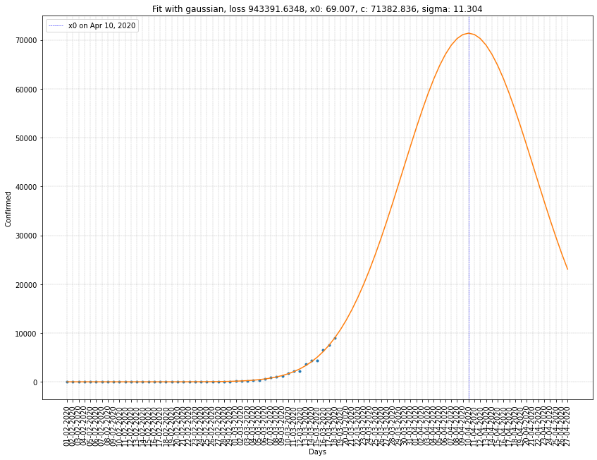
Gaussian regression summary
| Country | \(x_0\) | \(c\) | \(\sigma\) | loss |
|---|---|---|---|---|
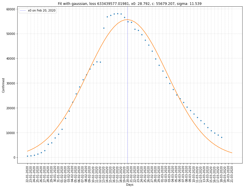
| China | 20/02/2020 | 55679 | 11.539 | 6.3x10⁸ |
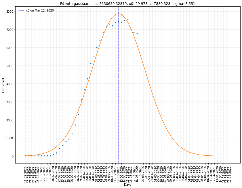
| South Korea | 12/03/2020 | 7880 | 8.551 | 3.3x10⁶ |
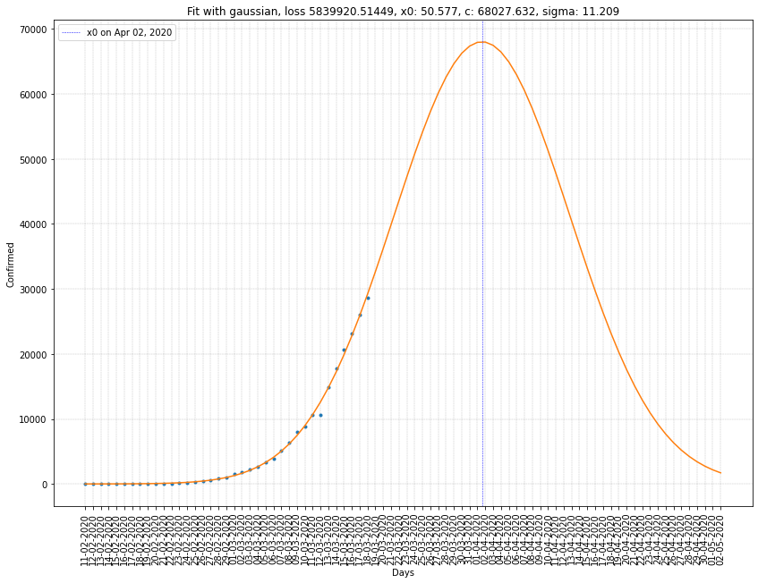
| Italy | 02/04/2020 | 68027 | 11.209 | 5.8x10⁶ |
| France | 10/04/2020 | 71382 | 11.304 | 9.4x10⁵ |
Here we can see that \(x_0\) is ten to twenty days greater than before. Which gives us a better estimation of the peak of the virus spread in France and Italy.
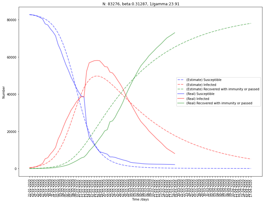
Modeling with SIR
On a different angle, we can also use a mathematical epidemic model to understand the trend of infection. Here we present the SIR model, for Susceptible Infected Recovered.
Constants
- \(N\): (fixed) population of N individuals
Time dependent functions
- \(S(t)\): susceptible but not yet infected cases
- \(I(t)\): the number of infected individuals
- \(R(t)\): count of recovered cases with immunity
Coefficients
- \(\beta\): the effective contact rate of the disease. An infected individual comes into contact with \(\beta N\) other individuals per unit time. \(\beta = \alpha \times p\) where \(\alpha\) is the total number of contacts per unit time and \(p\) is the risk of infection.
- \(\gamma\): the mean recovery rate. \({ 1 \over \gamma}\) is the mean period of time during which an infected individual can pass it on. If the duration of the infection is denoted \(D\), then \(\gamma = { 1 \over D}\), since an individual experiences one recovery in \(D\) units of time.
- \(R_0\): the basic reproduction number, is the expected number of individuals infected by one infectious case. \(R_0 = \beta \times D\) with \(\beta\) the effective contact rate and \(D\) the duration of the infection.
Differential equations
\[\begin{align} { d S \over d t} &= - { \beta SI \over N}\\ { d I \over d t} &= { \beta SI \over N}\ - \gamma I\\ { d R \over d t} &= \gamma I \end{align}\]What we know about Coronavirus
At the moment, the estimated basic reproduction number is betwen 2.5 and 5. We also know the population for each country but we won’t use them in this particular model. With the data taken from John Hopkins University, we can get all three temporal functions. The estimated days of infection is between 15 and 20 with a mean incubation period of 5-6 days.
Let’s fit the data to multiple countries.
Fitting China to SIR model
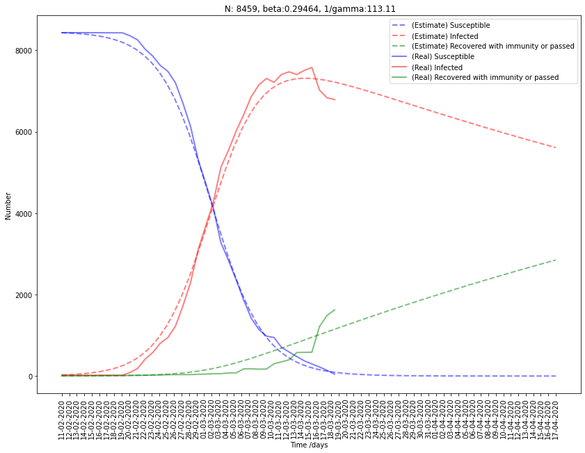
Fitting South Korea to SIR model
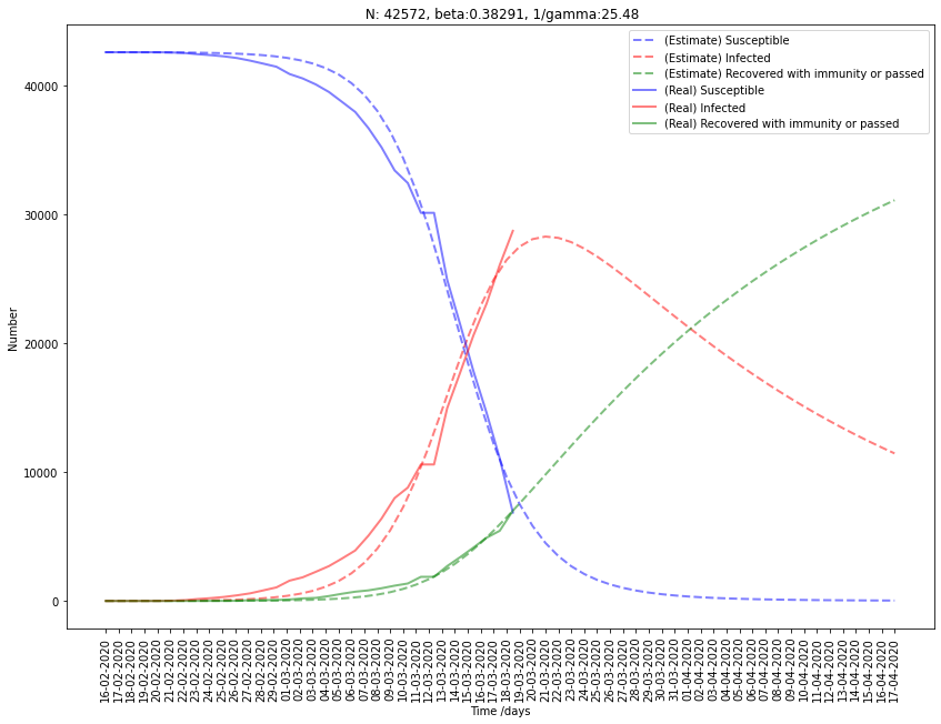
Fitting Italy to SIR model
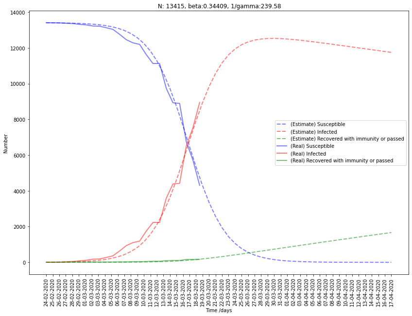
Fitting France to SIR model
SIR summary
| Country | \(N\) | \(\beta\) | \(\gamma\) | \(D\) | \(R_0\) (\(\beta D\)) |
|---|---|---|---|---|---|
| China | 83276 | 0.313 | 0.041 | 23.9 | 7.48 |
| South Korea | 8459 | 0.295 | 0.0088 | 113.1 | 33.3 |
| Italy | 42572 | 0.383 | 0.0395 | 25.5 | 9.75 |
| France | 13415 | 0.344 | 0.0042 | 239.6 | 82.4 |
First, we can drop the estimation of South Korea and France because the results for \(\gamma\) seem pretty wrong. Indeed, it gives us a really high period of infection \(D\) (\(\gamma = { 1 \over D}\)).
For Italy, the fit seems a little erroneous because the infected cases will surely continue to increase in the next few days before starting to decrease. This bad estimation may come from the fitting method I used.
Finally, for China, despite that the loss is not optimal, the results are not too bad. The \(R_0\) estimated for China is 7.5, around two times geater than the one estimated by experts. In fact, SIR doesn’t modelize the incubation period, and while and individual in incubation may be infectious, this model can be improved.
Here is a graph from annals.org, showing the cumulative distribution of Covid-19 incubation period.
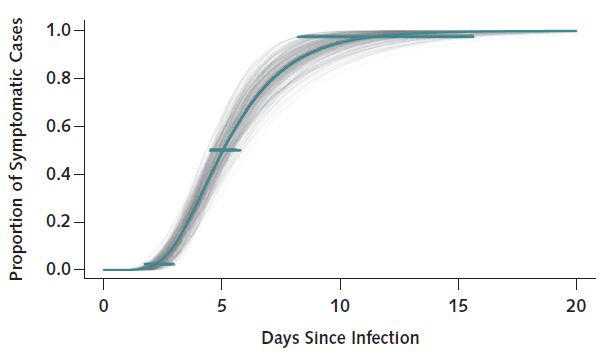
One way to go forward would be to test the SEIR model that takes the incubation period into account.